Making Polygons Morph and Float
For my collaboration with composer Katie Balch, titled still life, we wanted to find ways to abstract the sound and video we were recording in the forests of Connecticut. Here I describe one strategy that I used to make hundreds of polygons morph–transitioning between different video scenes. The final video will be spread out over 3 16:9 screens/projector in front of/around the audience. All the computation and rendering described below was done in openFrameworks: a creative coding library for C++.
Canny Edge Detection & Contour Finder
Canny edge detection is a common first step in many classic computer vision algorithms (I say classic because now most CV is ML/CNN based). It finds distinct changes in the image (usually based on brightness) and returns another rasterized image showing where these “edges” are detected. I then use a “contour finding” algorithm to transform the edges in the raster to vector data, returned in the form of lines (i.e., “contours”, i.e., a series of x,y points that can be connected in order). In order to create a polygon from a contour, I just connected the last point back to the first point.
The parameters of the canny algorithm have a pretty big affect on how many polygons are found (the main two parameters are two thresholds for a hysteresis gate). Because I want all the analyzed frames to end up with approximately the same number of polygons, I set a target number and then do a grid search to find what combination of parameters will be nearest to the target (or the first that is within a given threshold of the target: 5%). For each subsequent frame, I begin the grid search from the previous frame’s successful parameters because adjacent frames are usually pretty similar. If the previous frame’s parameters produce a number of polygons within the threshold of the target, then I don’t pursue the grid search.
Polygon Processing
For each frame, I first iterate over the polygons and process them in various ways:
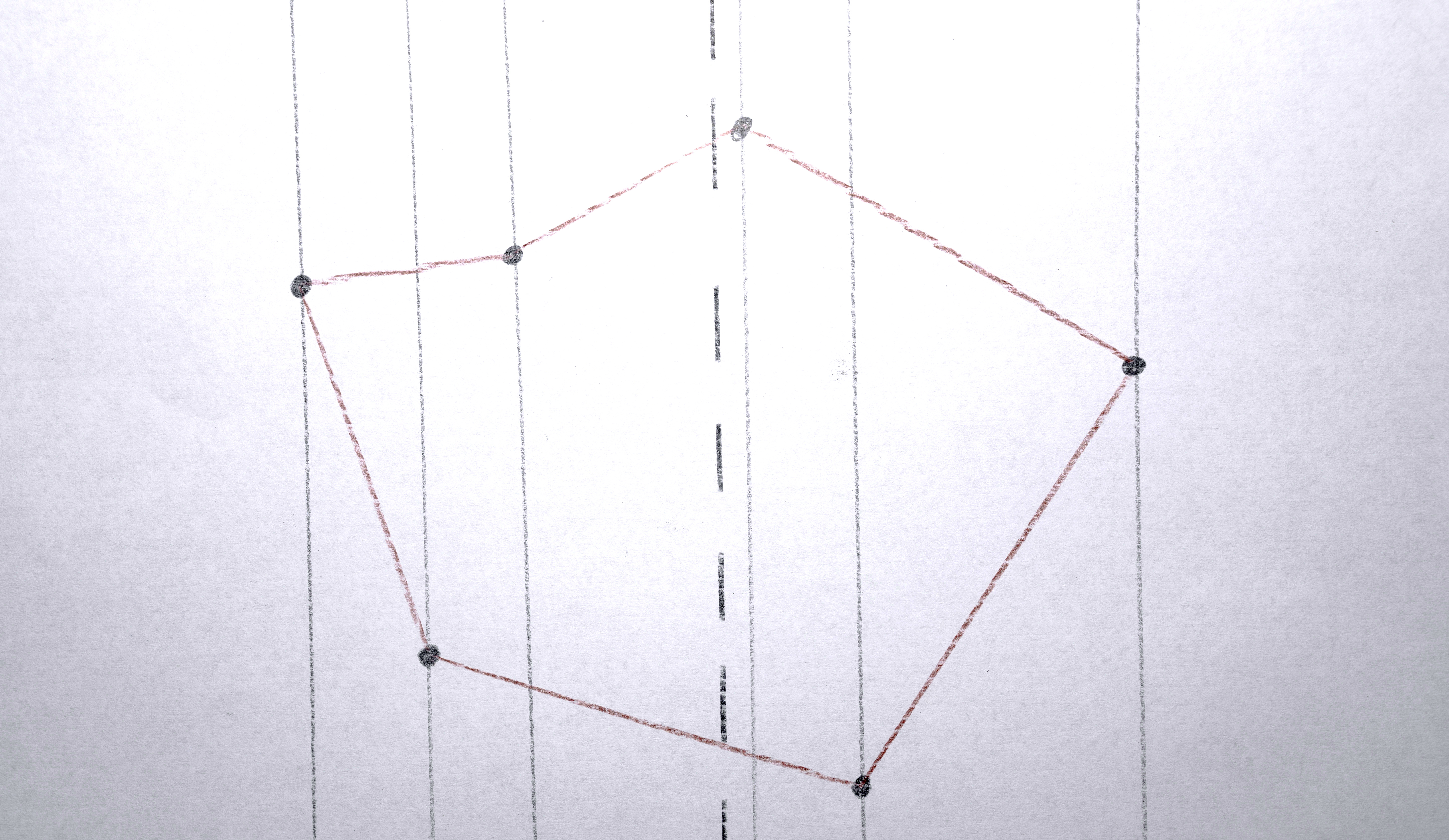
1. Check if a polygon is too close to an “edge” by checking if any of the polygon’s points are within a threshold of one of any vertical edge of any of the 3 screens. The way the algorithm works, polygons are often near these edges and I just don’t like how they look.
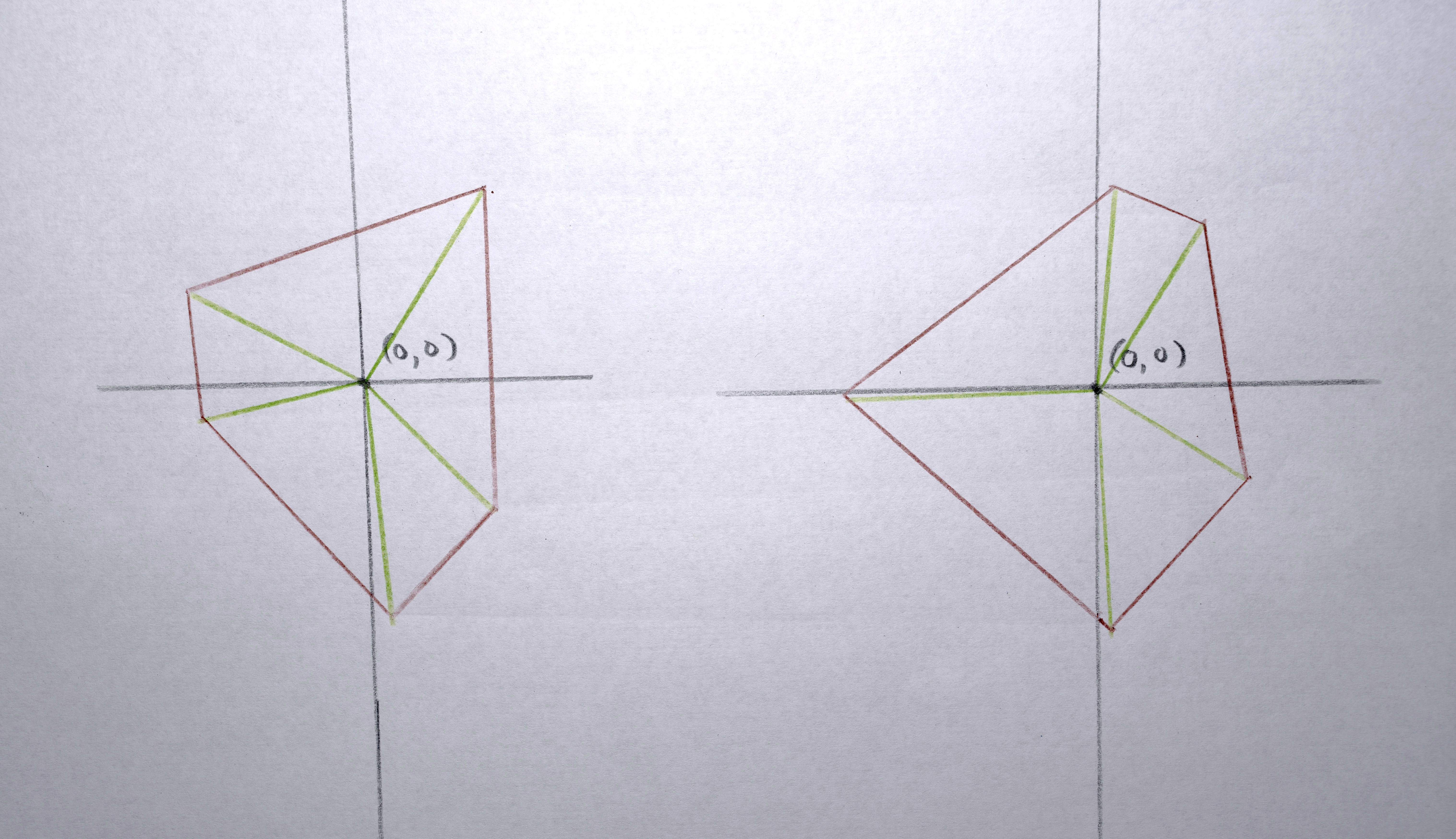
2. Compute the “centroid” of the points of the polygon to give the polygon a single x,y position to represent it.
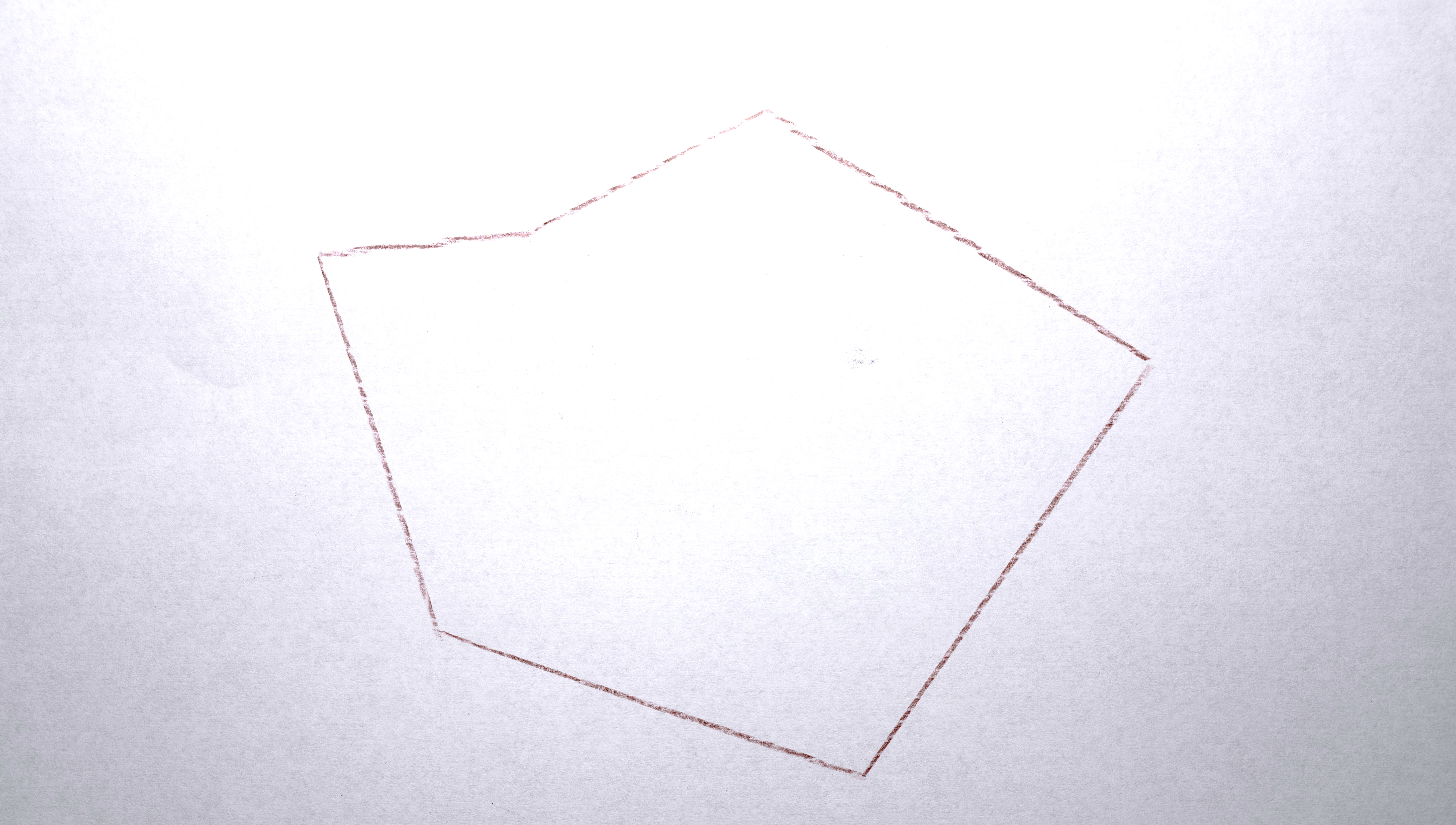


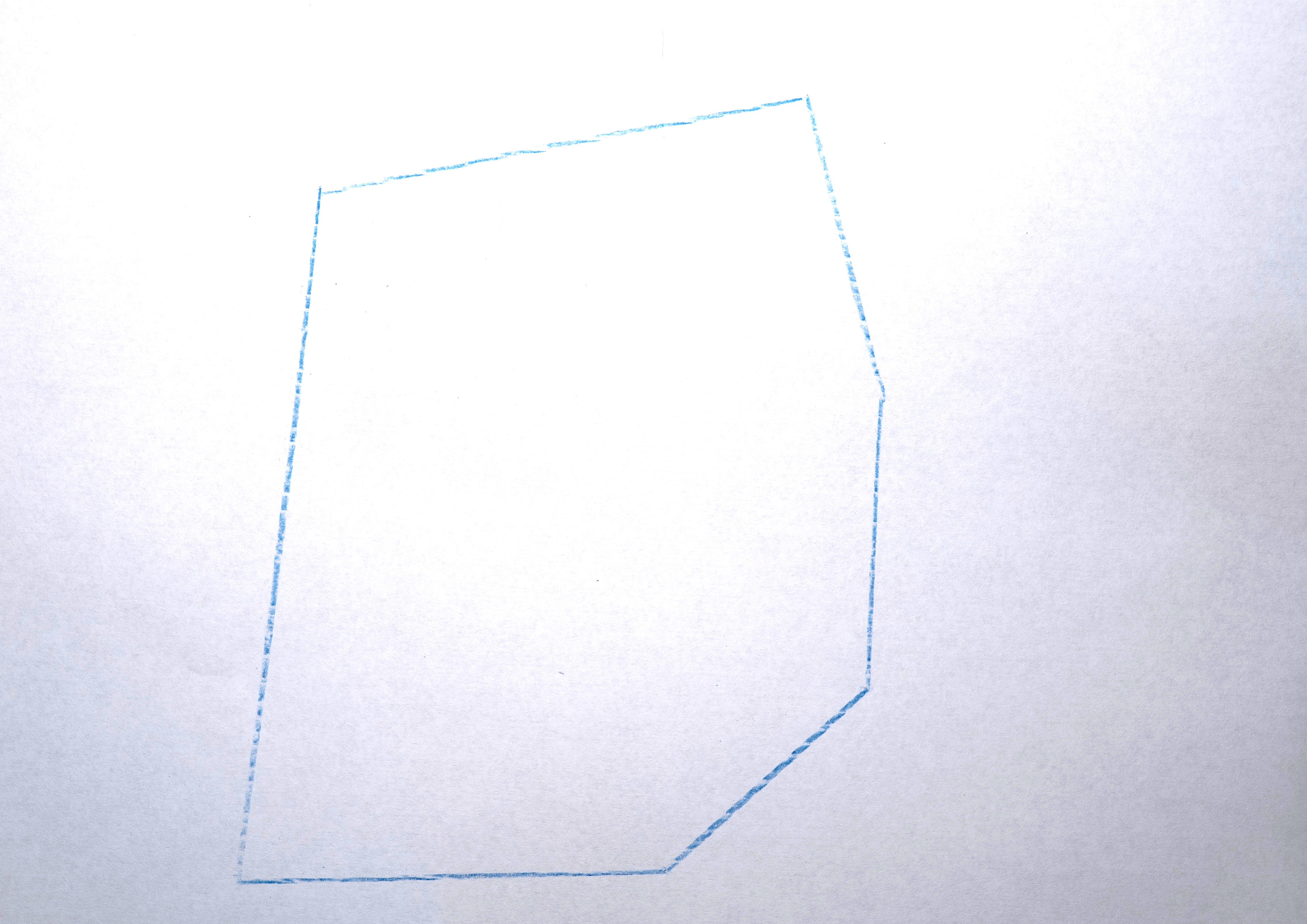
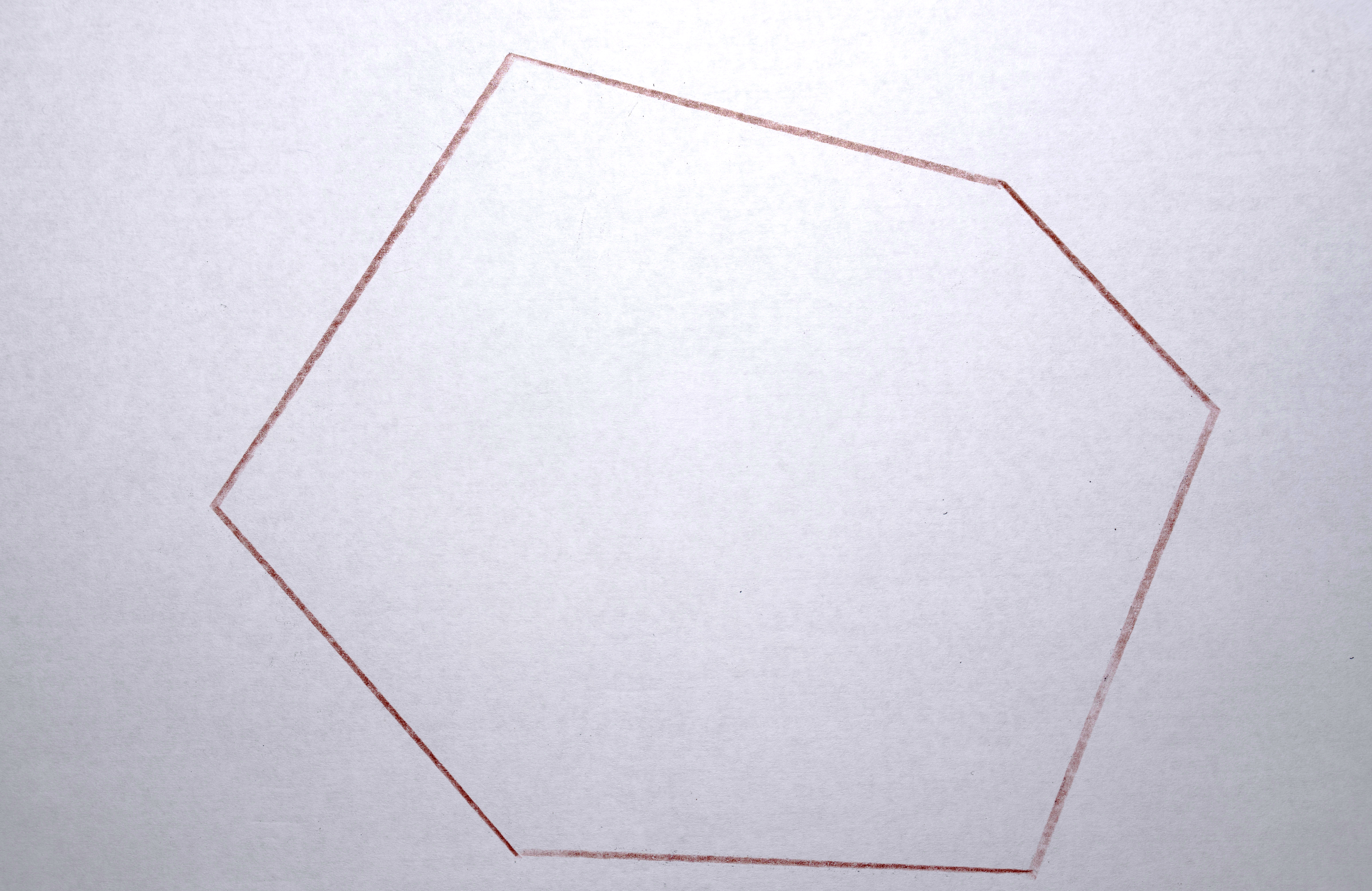
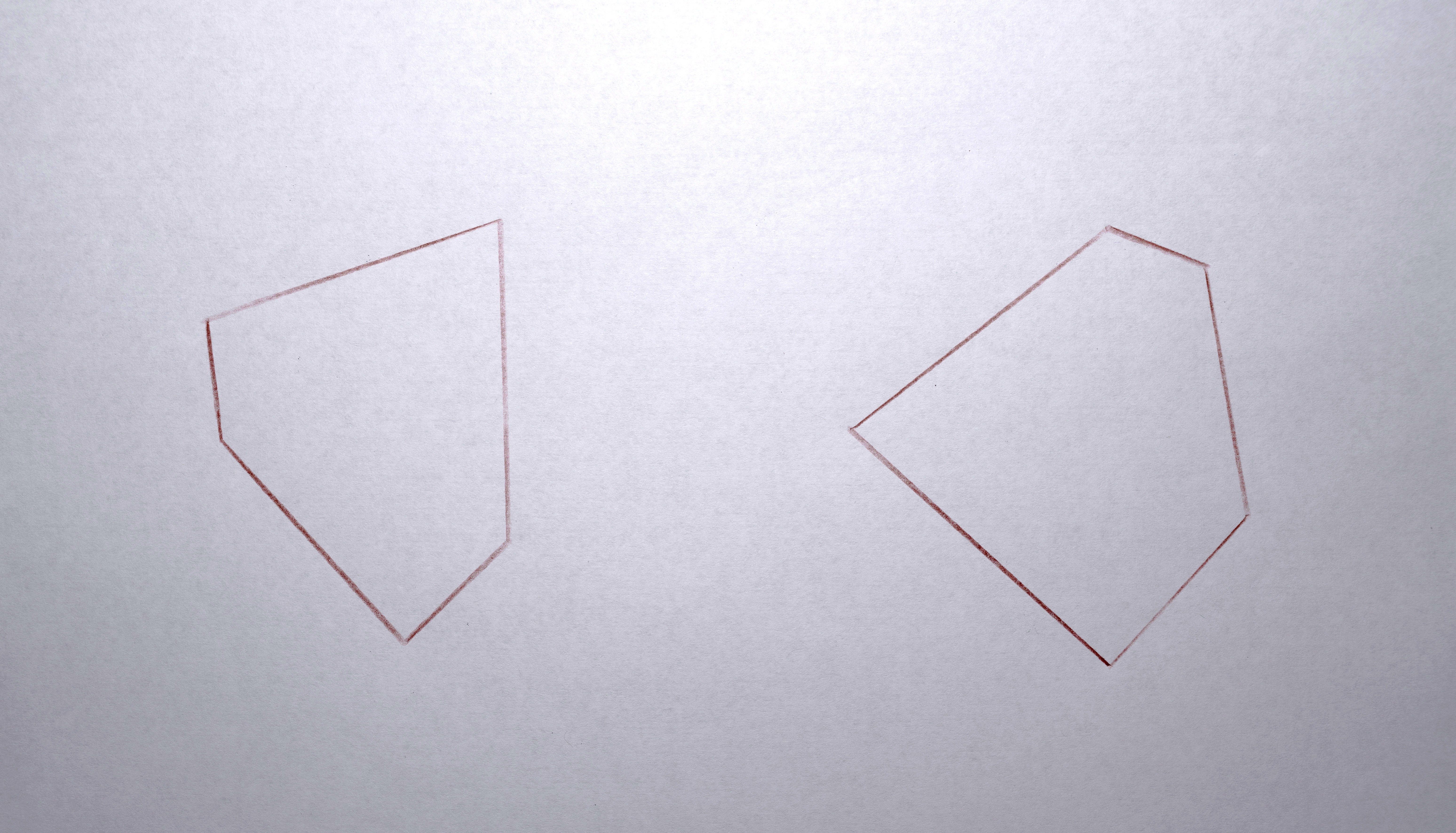
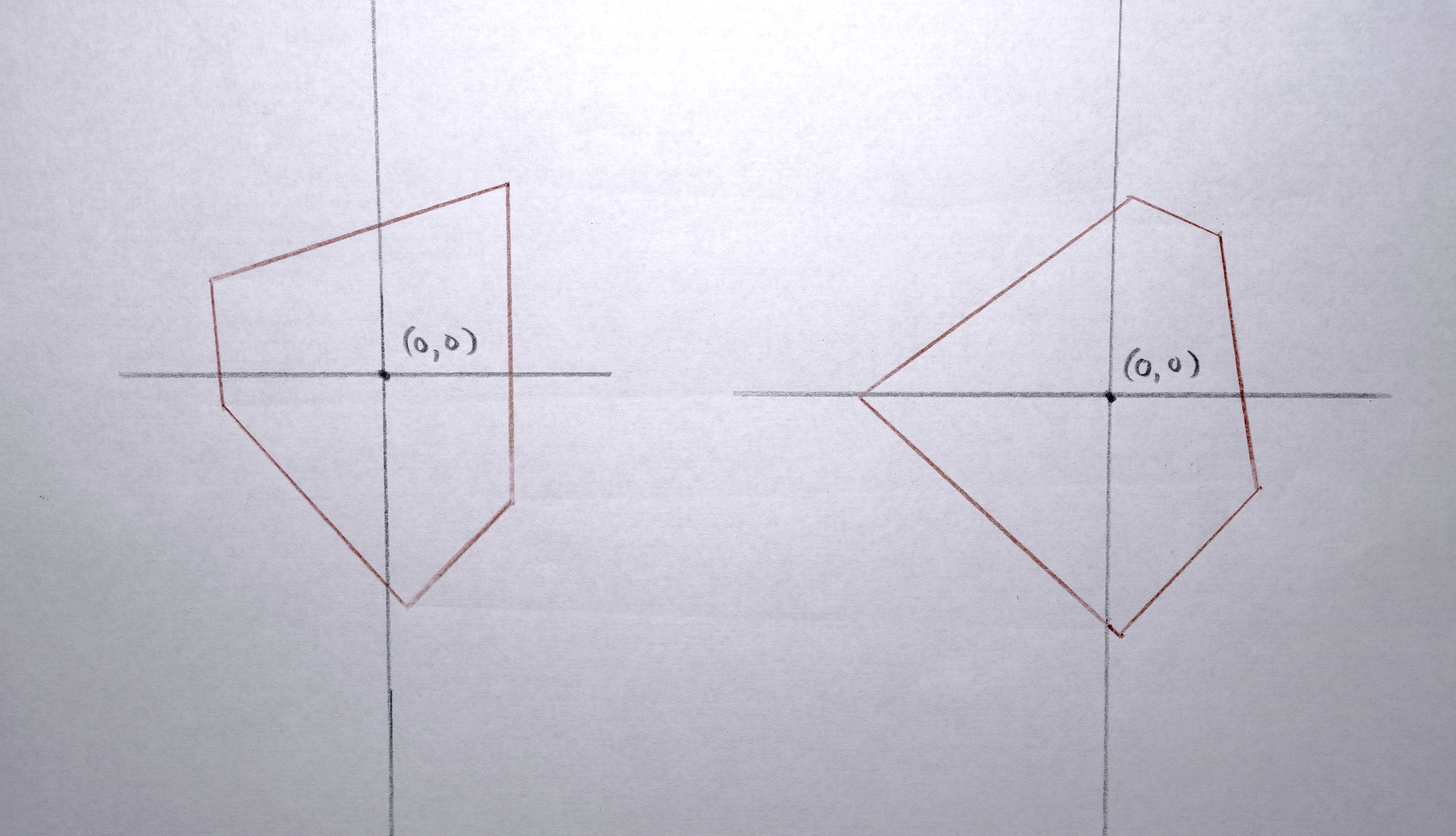
3. Transform each polygon into a convex hull because it nicely abstracts the shapes by making them simpler.
4. Assign the polygon a color taken from the original image at the x,y position of the centroid computed in #1.
5. Create a vector of “descriptors” to represent the polygon when determining how “similar” it is to other polygons (this will be needed later). The elements in the vector are: [ centroid x, centroid y, convex hull area, color red, color green, color blue ]. Usually the (unnormalized) weights of these dimensions is [ 1, 1, 0, 0, 0, 0], so what is being compared when considering “similarity” is actually just x and y position. Later, only area is considered, and in some tests, color was also included.
6. Smooth out the polygons a bit to removes sharp corners.

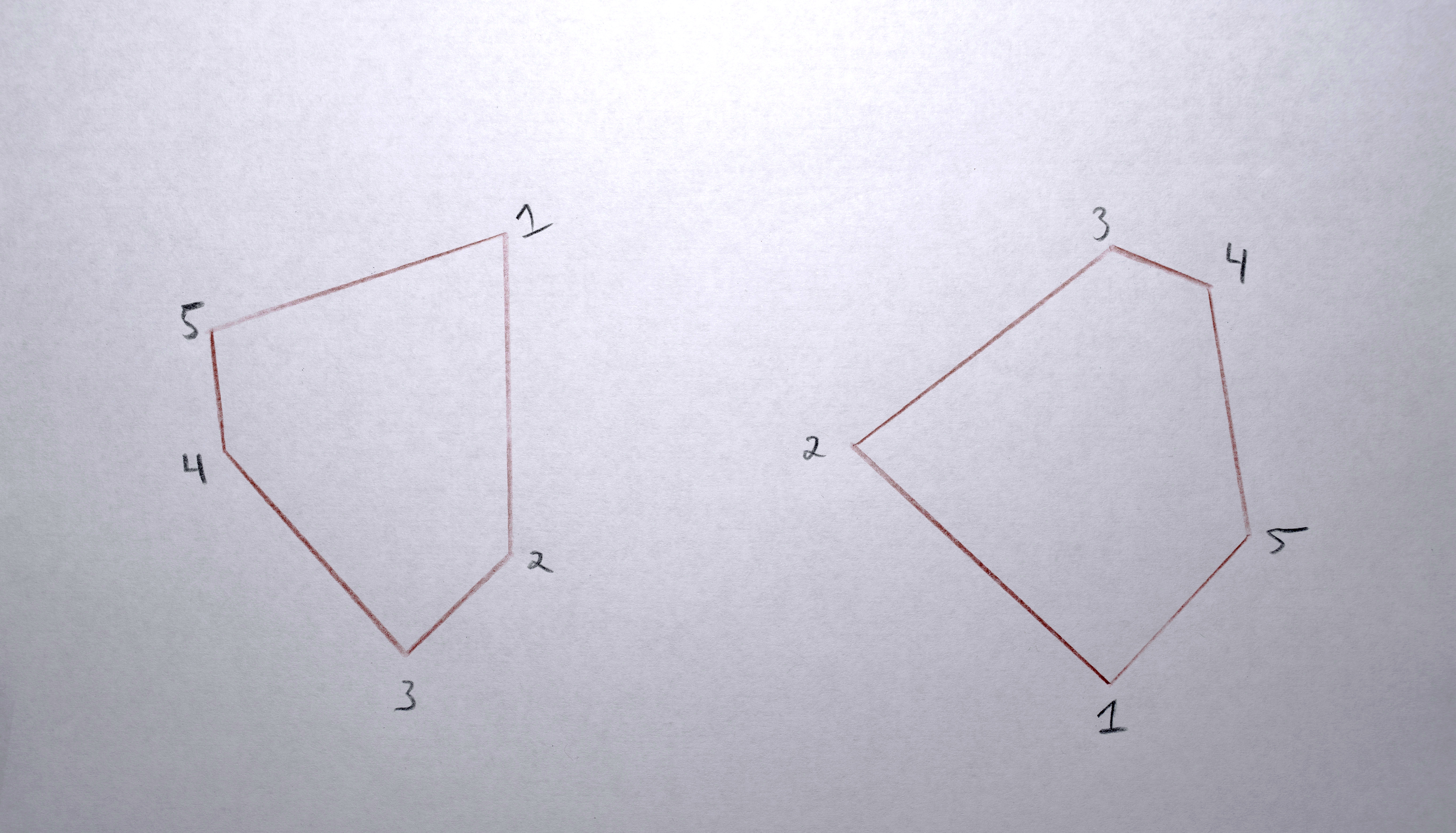
Connecting Polygons into Sequences
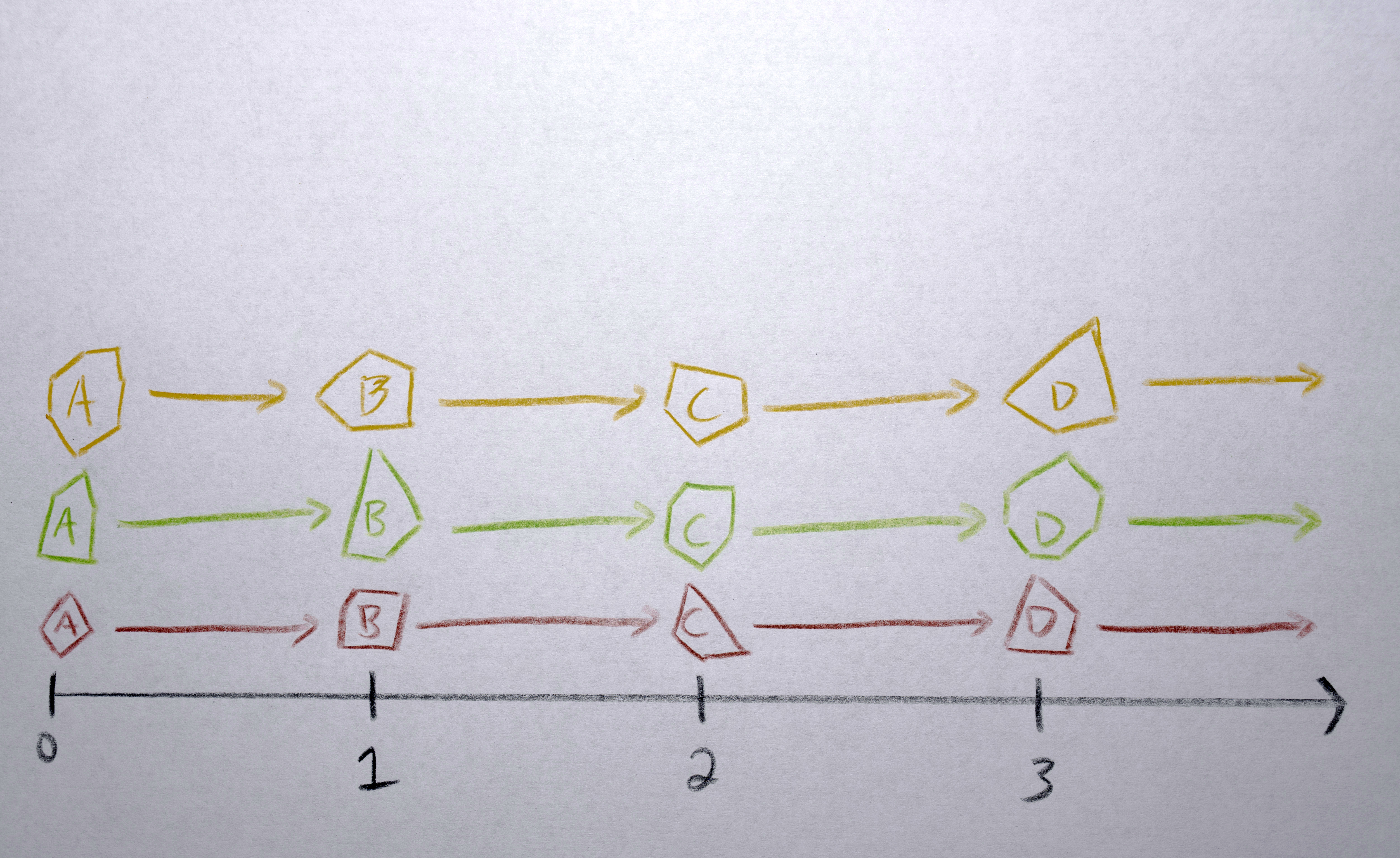
I next created sequences of polygons connecting one in every frame to a “similar” polygon in the next frame: the one it will morph into. Some frames had different numbers of polygons in them so below you’ll see where I had to “fade in” or “fade out” (using opacity) to match the number of polygons need for a given frame.
All the polygons in the first frame are the start of a sequence. For each subsequent frame:
1. Gather the descriptor vectors of the polygons active in the previous frame ("f-1"). Standardize the vectors to a mean of 0 and standard deviation of 1.
2. Gather the descriptor vectors of the polygons in the current frame ("f") and scale them according to the statistics determined when standardizing the vectors of the “still active polygons”.
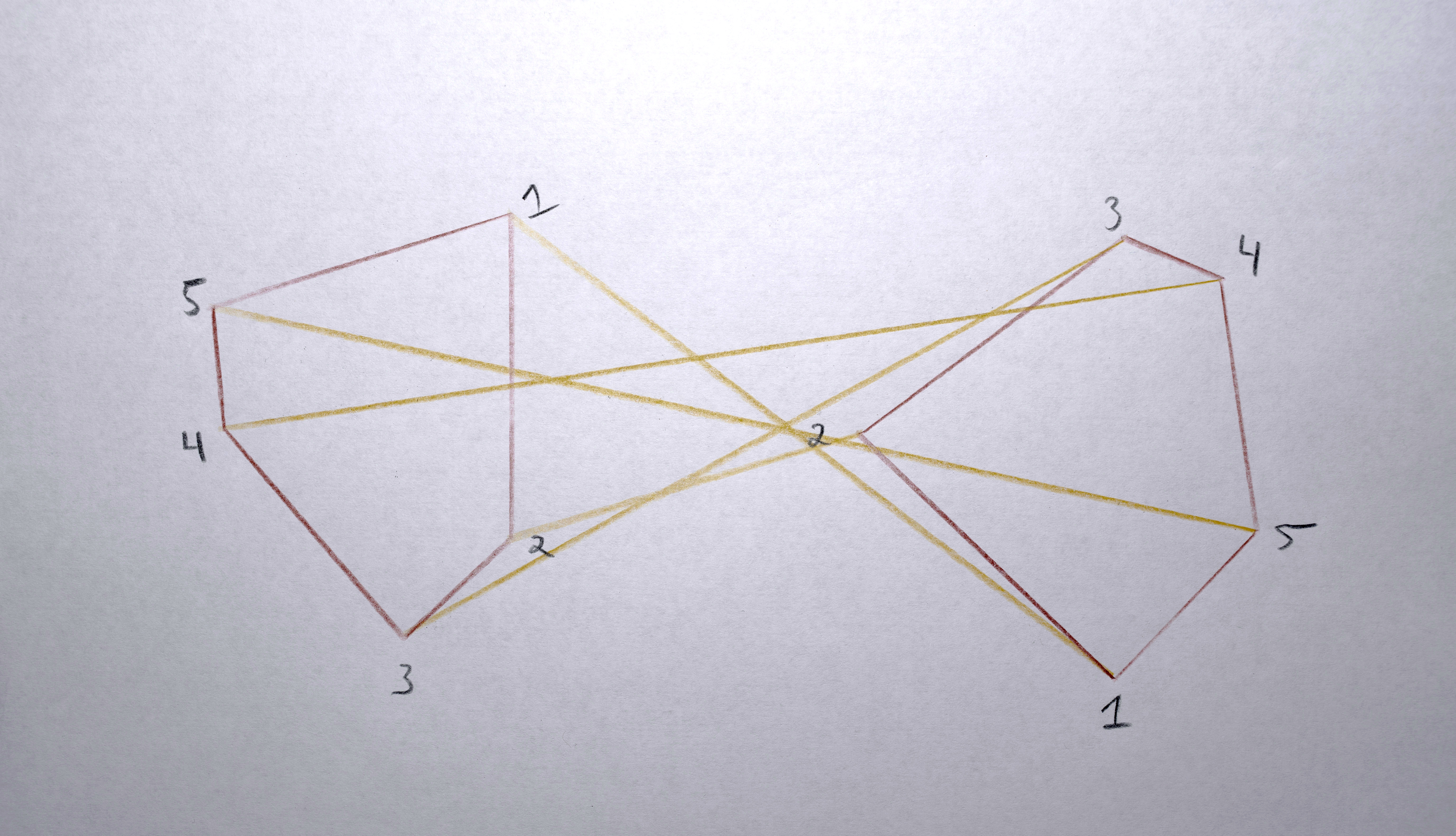
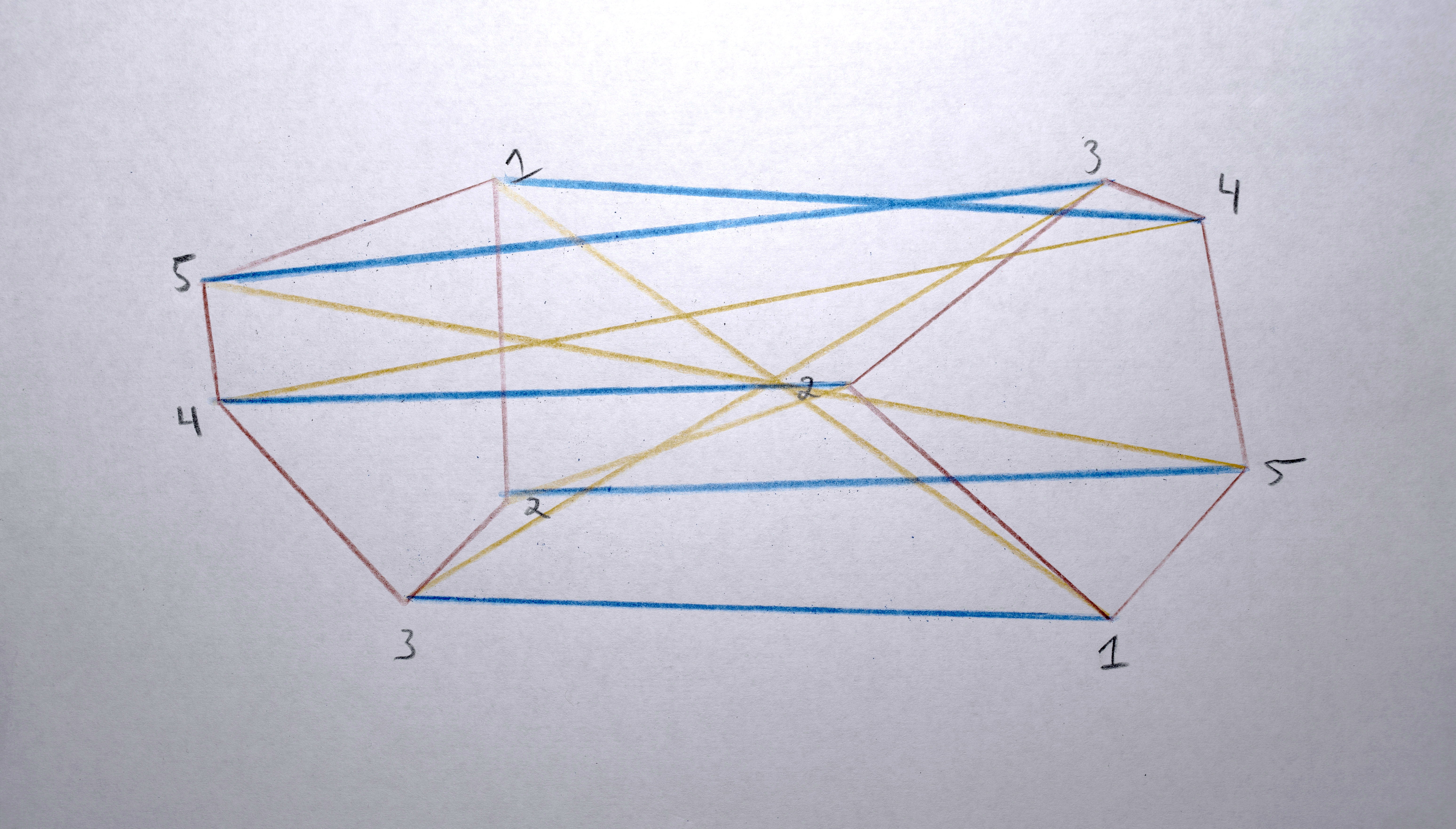
3. Build a “distance matrix” (aka. “cost matrix”) by computing the “distance” (usually euclidean distance in x,y space between the centroids) from every polygon in A and to every polygon in B.


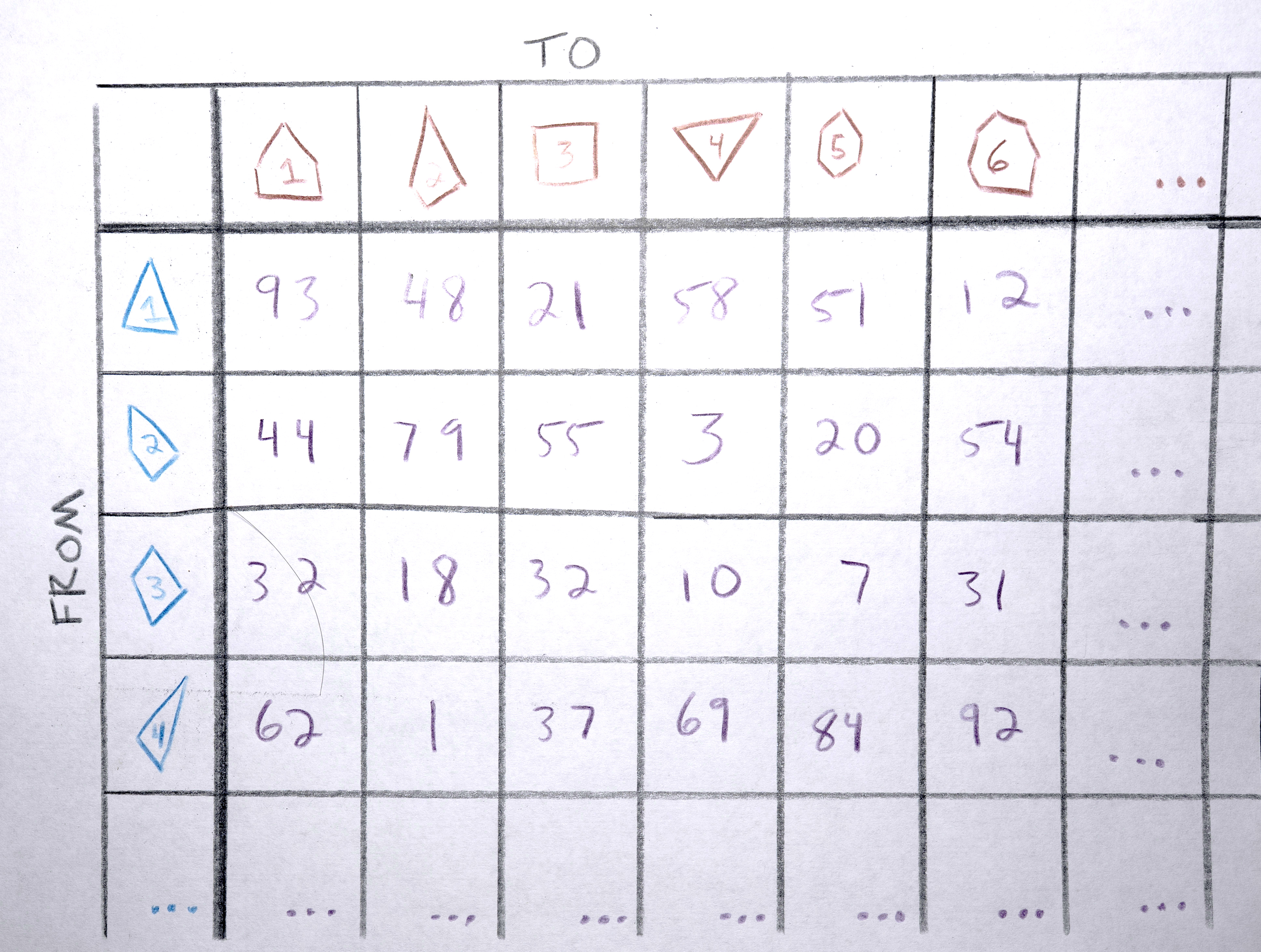

4. Match each polygon in A to a polygon in B by solving the distance matrix using the Munkres algorithm (an optimal solution to the linear assignment problem) such that the total distance moved by all polygons is minimized. This should result in polygons that in about the same spot in A as they are in B morph into each other. Any polygons in A that don’t get paired with a polygon in B are terminated (in the resulting video, they’ll start fading out at this point). Any polygons in the B that don’t get paired with a polygon from A starts a new sequence. There will never be both unpaired polygons from A and unpaired polygons from B. If there are the same number of polygons in both, the distance matrix will be a square and each polygon will get paired. If the distance matrix is a rectangle (either wider than it is tall or taller than it is wide), some polygons won’t get paired (only as many as one of the sides is longer than the other).
When moving between images that are similar, using x and y and maybe area as the descriptor vector makes sense for trying to minimize visual movement (of course it will never be perfect, giving the jittering variations that make it so appealing!). When moving between images that are not similar (especially if they’re on a different one of the 3 screens), it doesn’t make sense to use x or y as a descriptor vector because it’s going to have to travel so far, the “similarity” won’t be at all perceivable. I’ve used area and color as the measure of “similarity” in these cases (when rendering, I specify exactly which frames should use this alternative descriptor vector by modifying the descriptor vector weights before constructing the distance matrix).
Preparing Polygons for Morphing
Once those sequences are created, for each sequence:
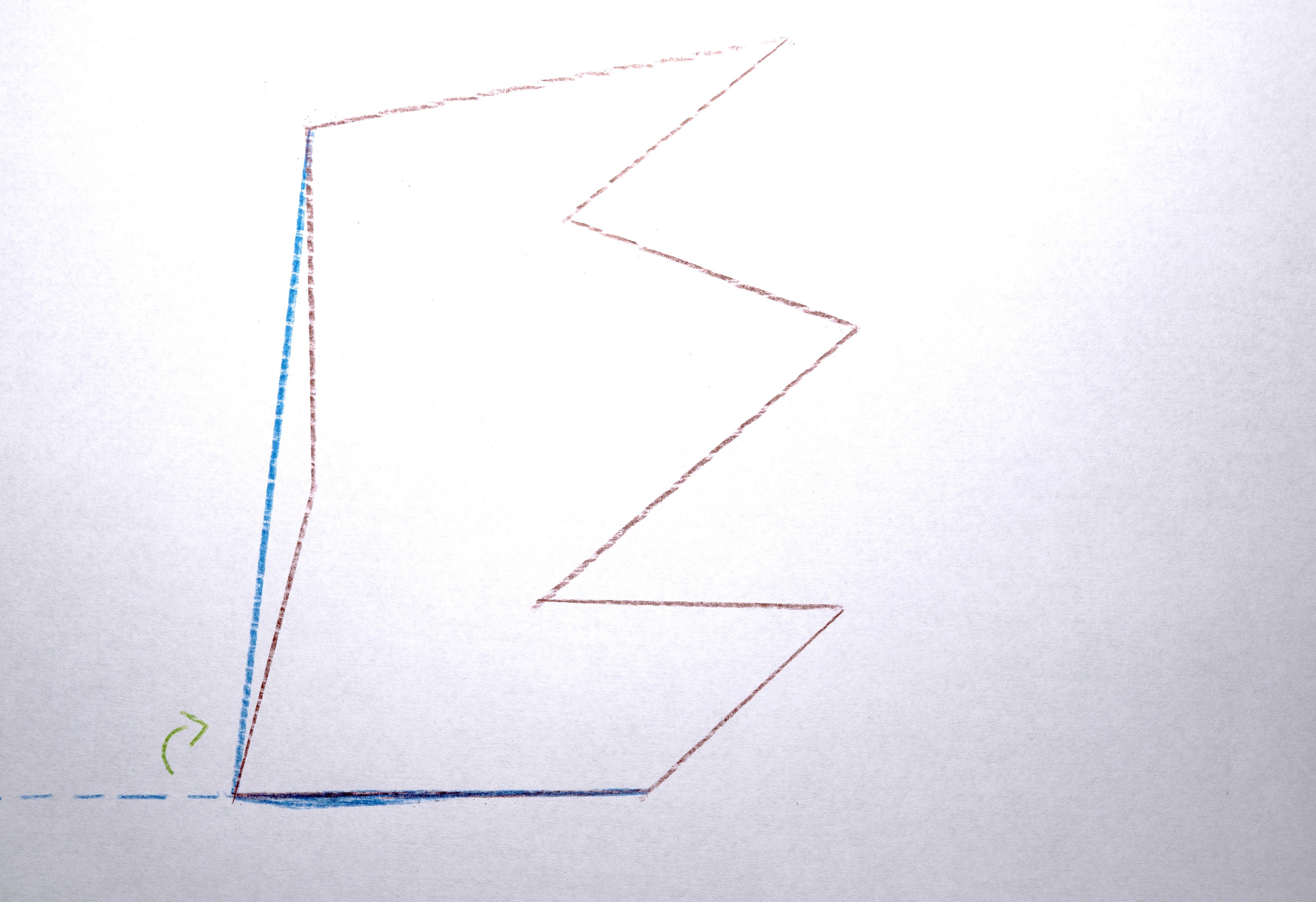
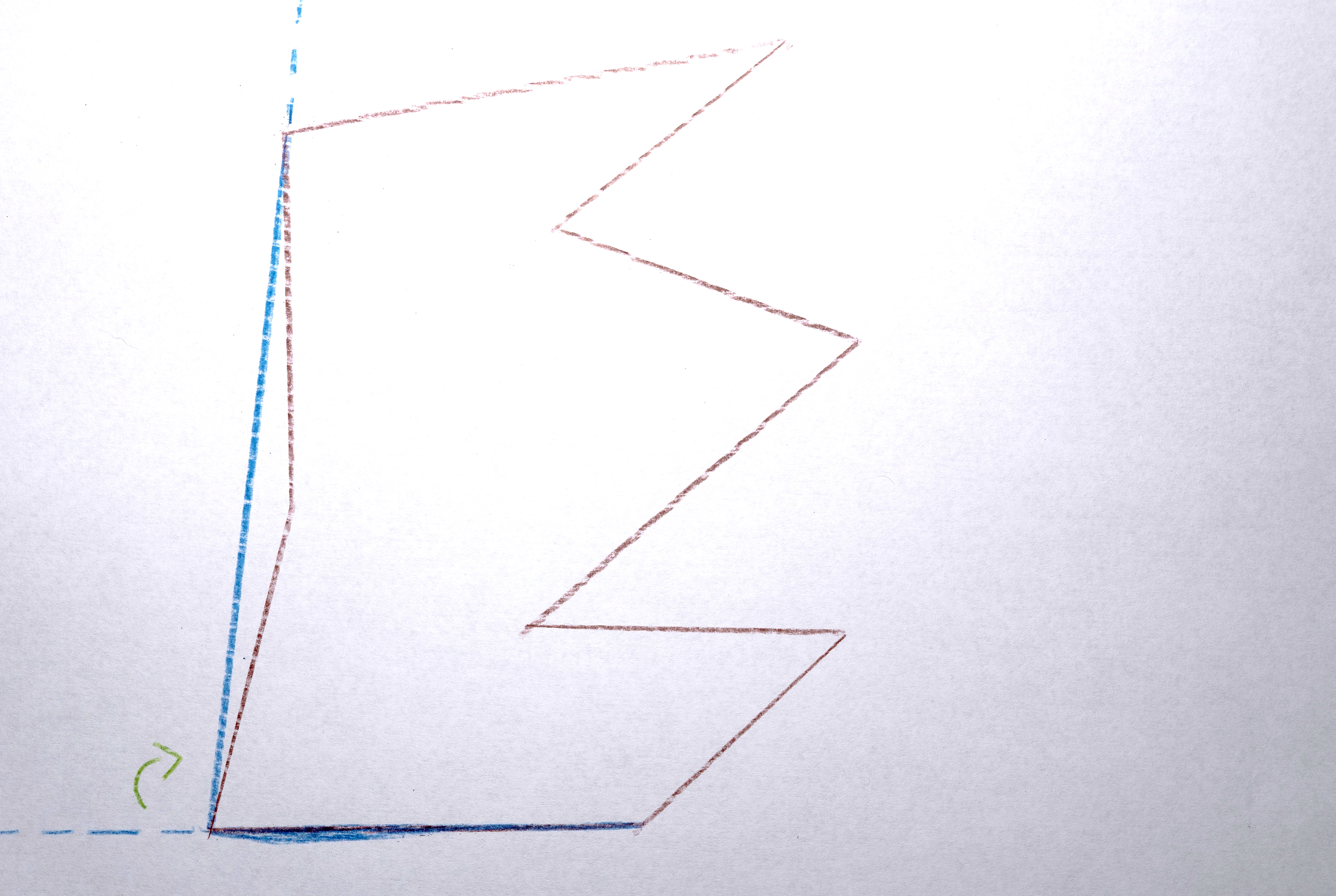
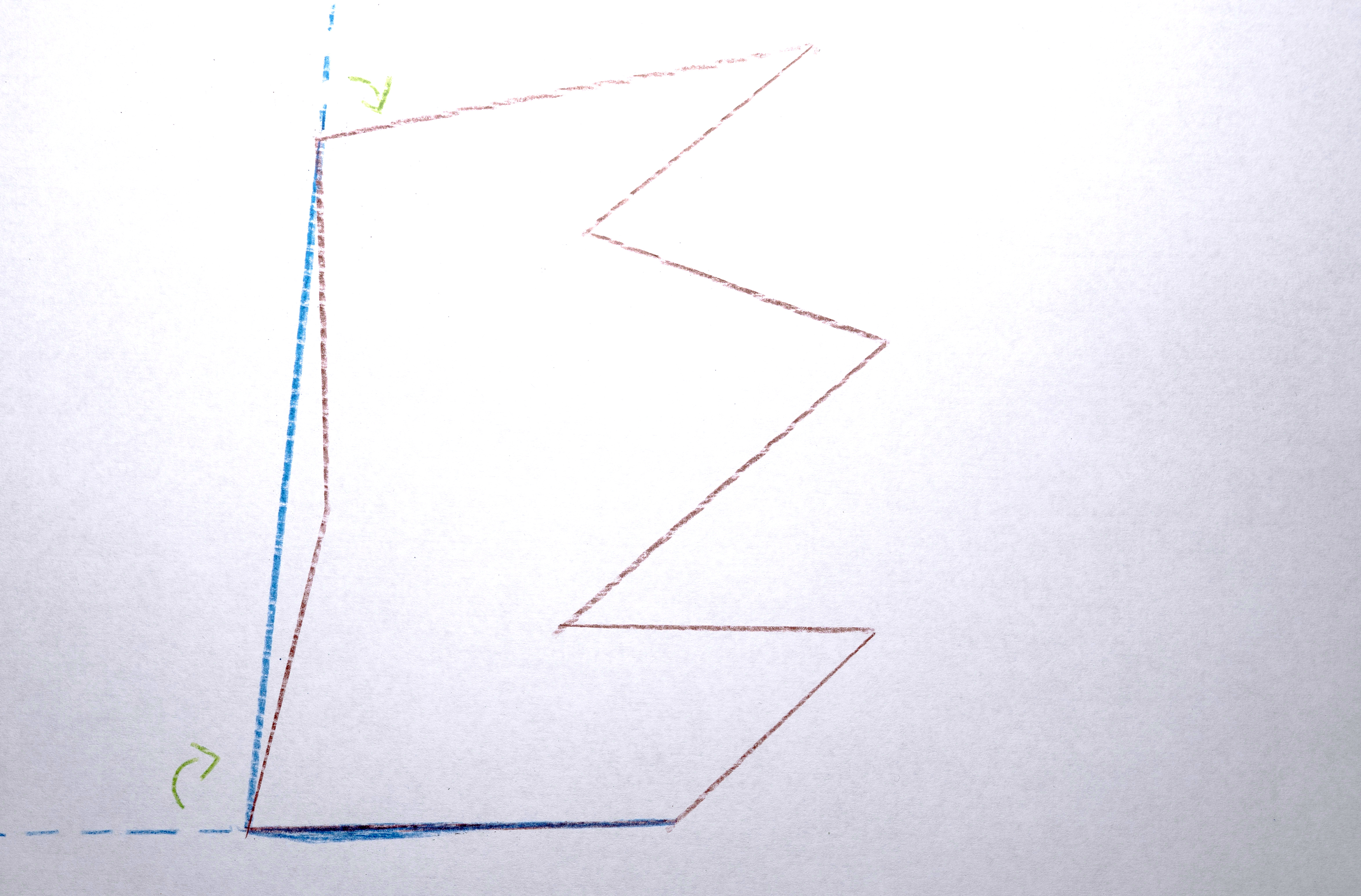
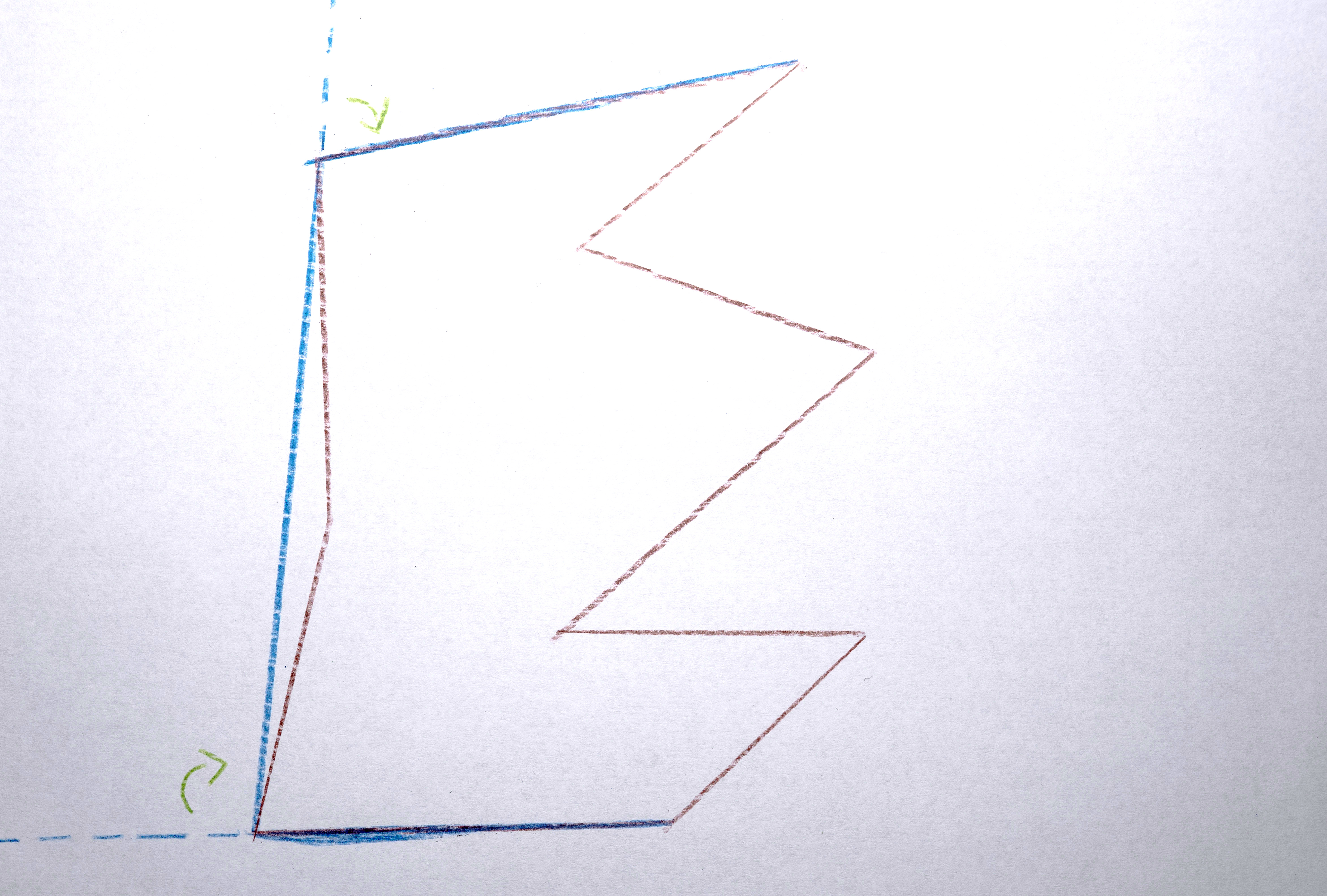
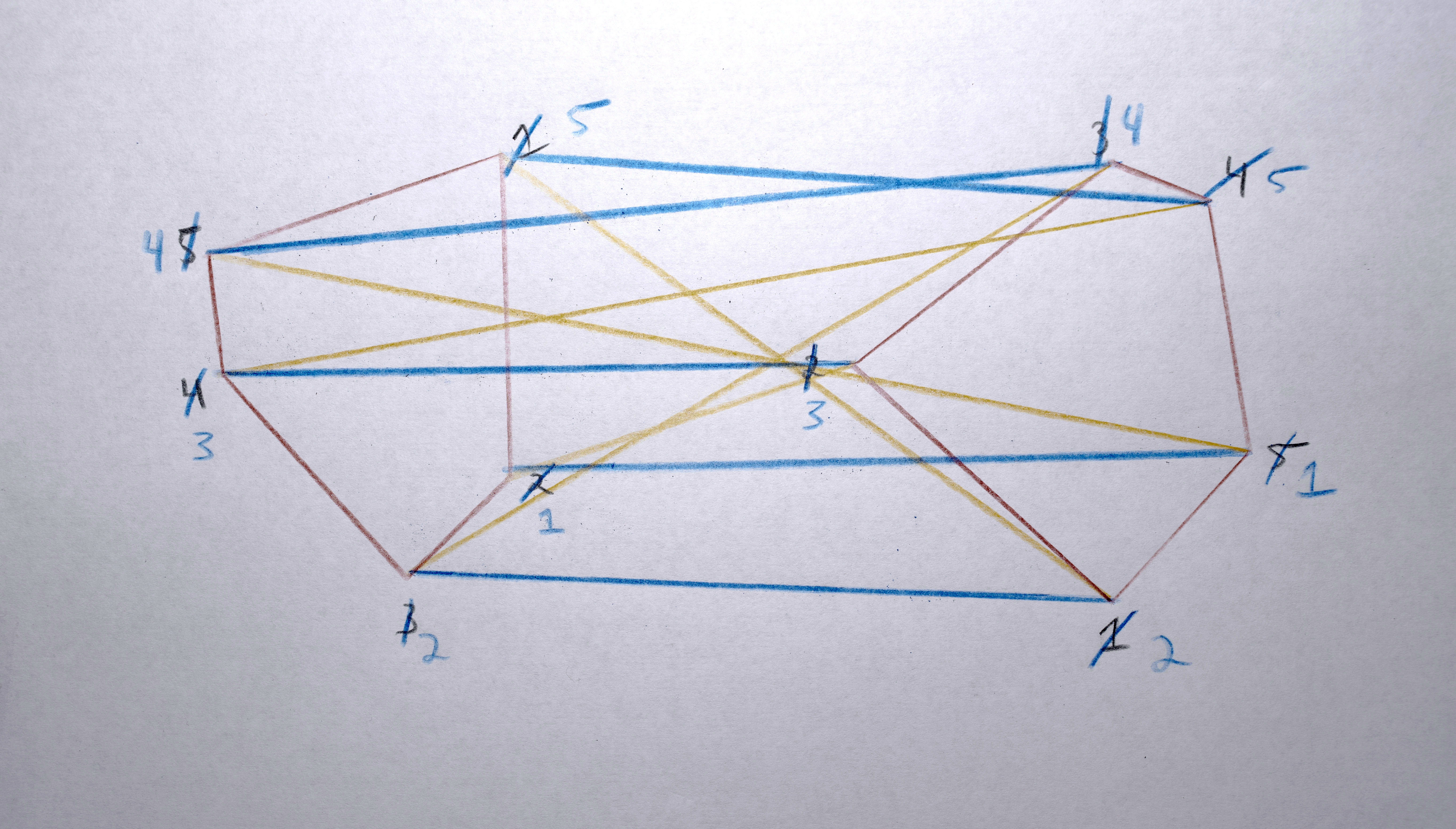
1. Find which the polygon in the sequence has the the most points creating its perimeter.
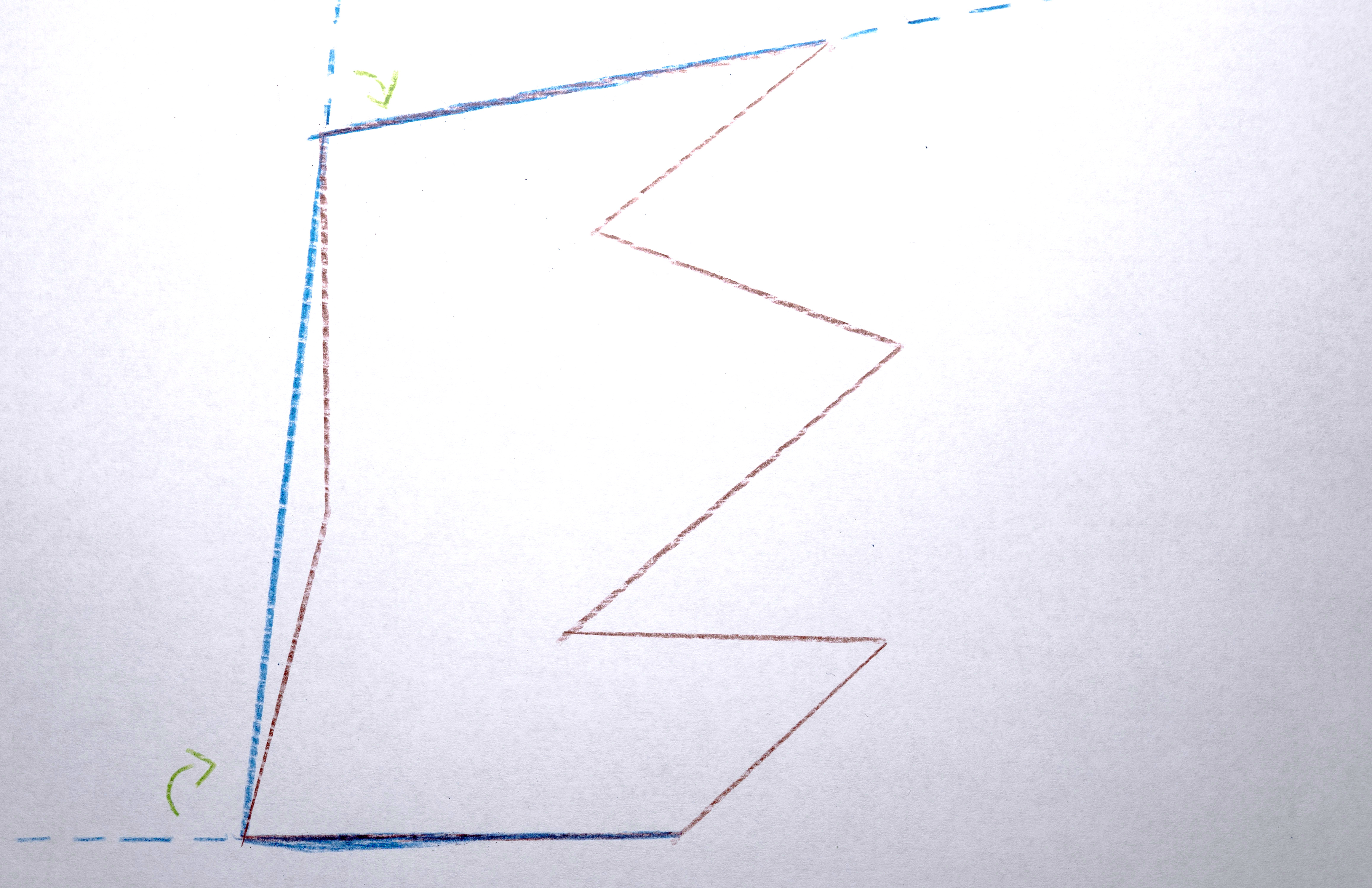
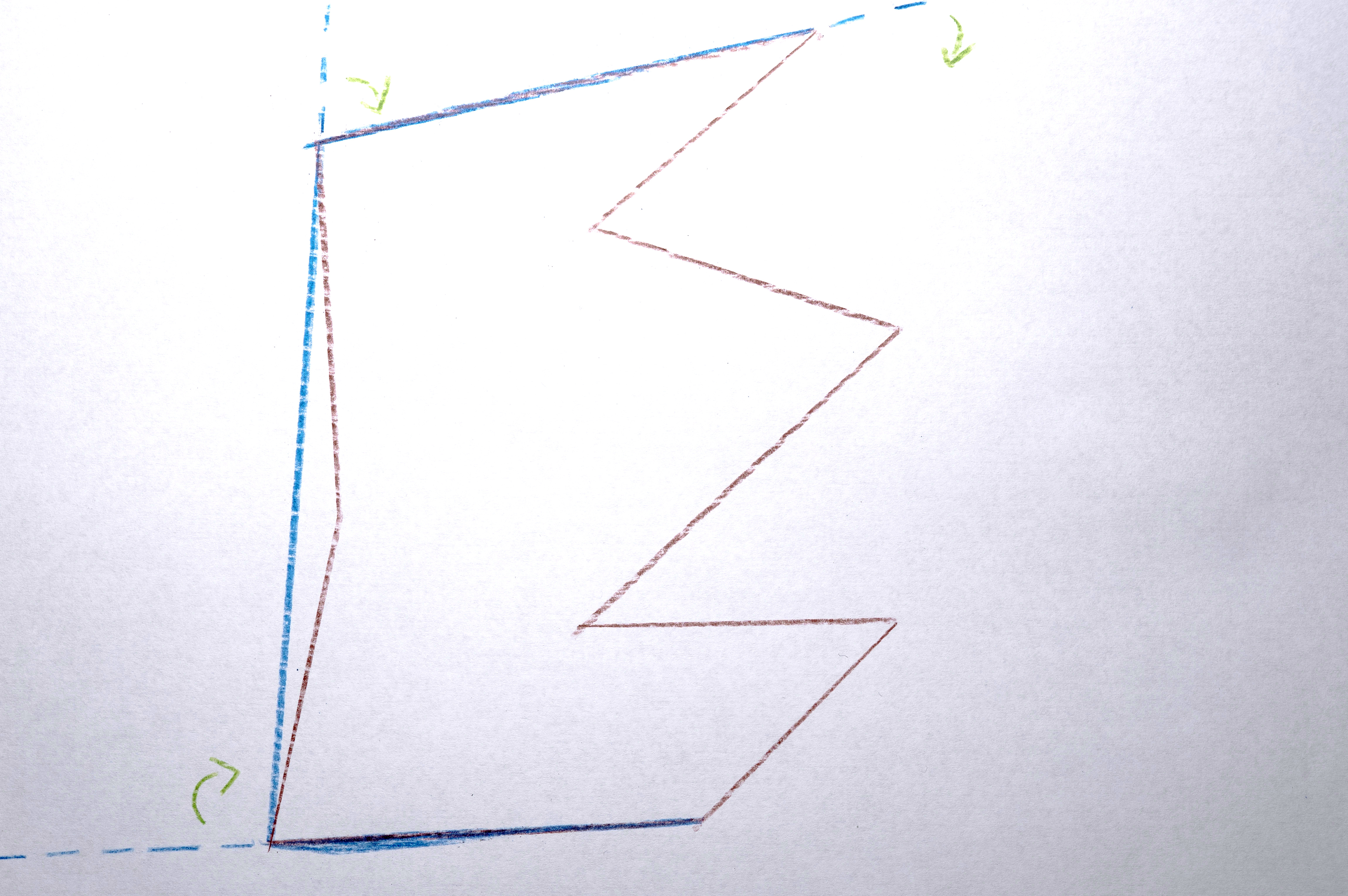
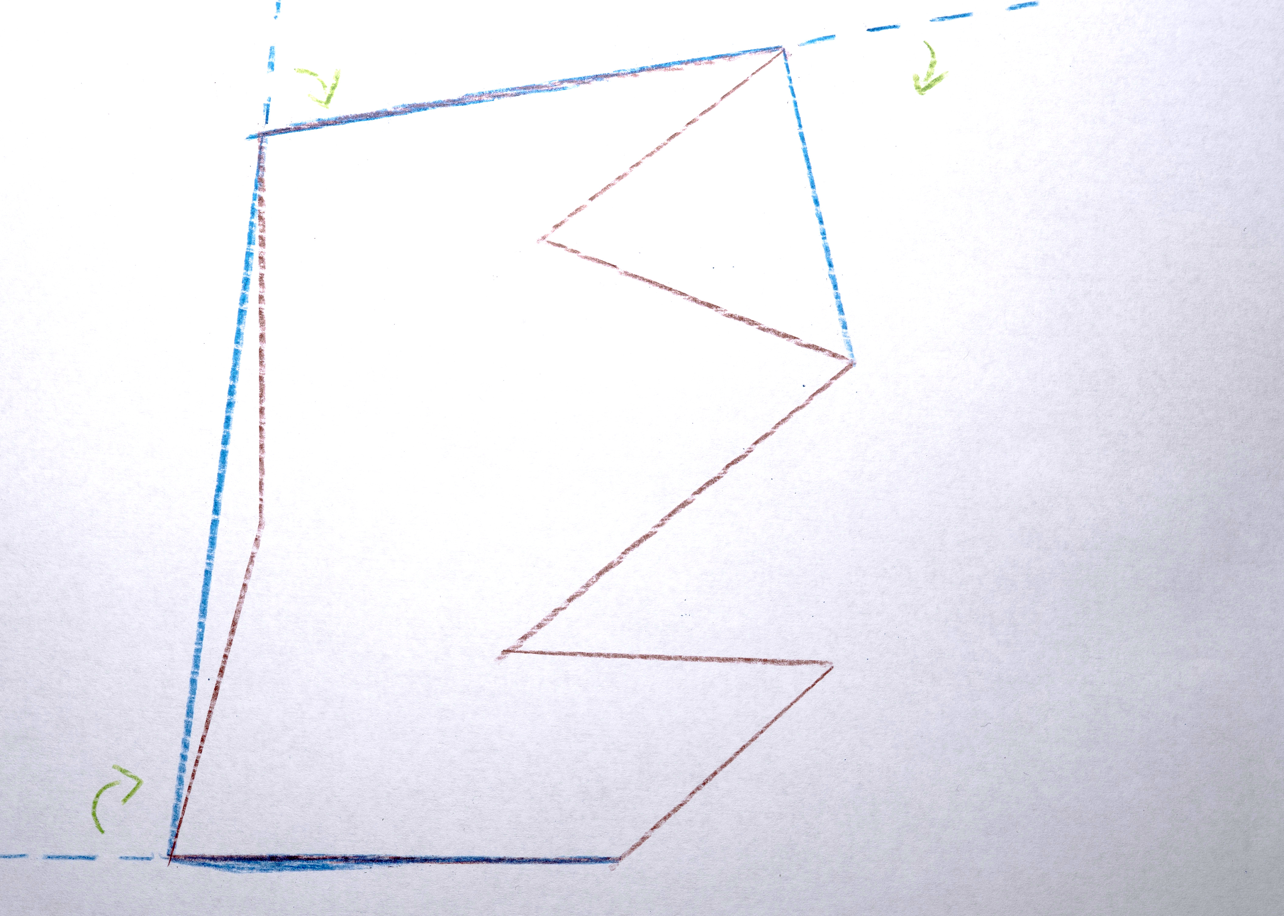
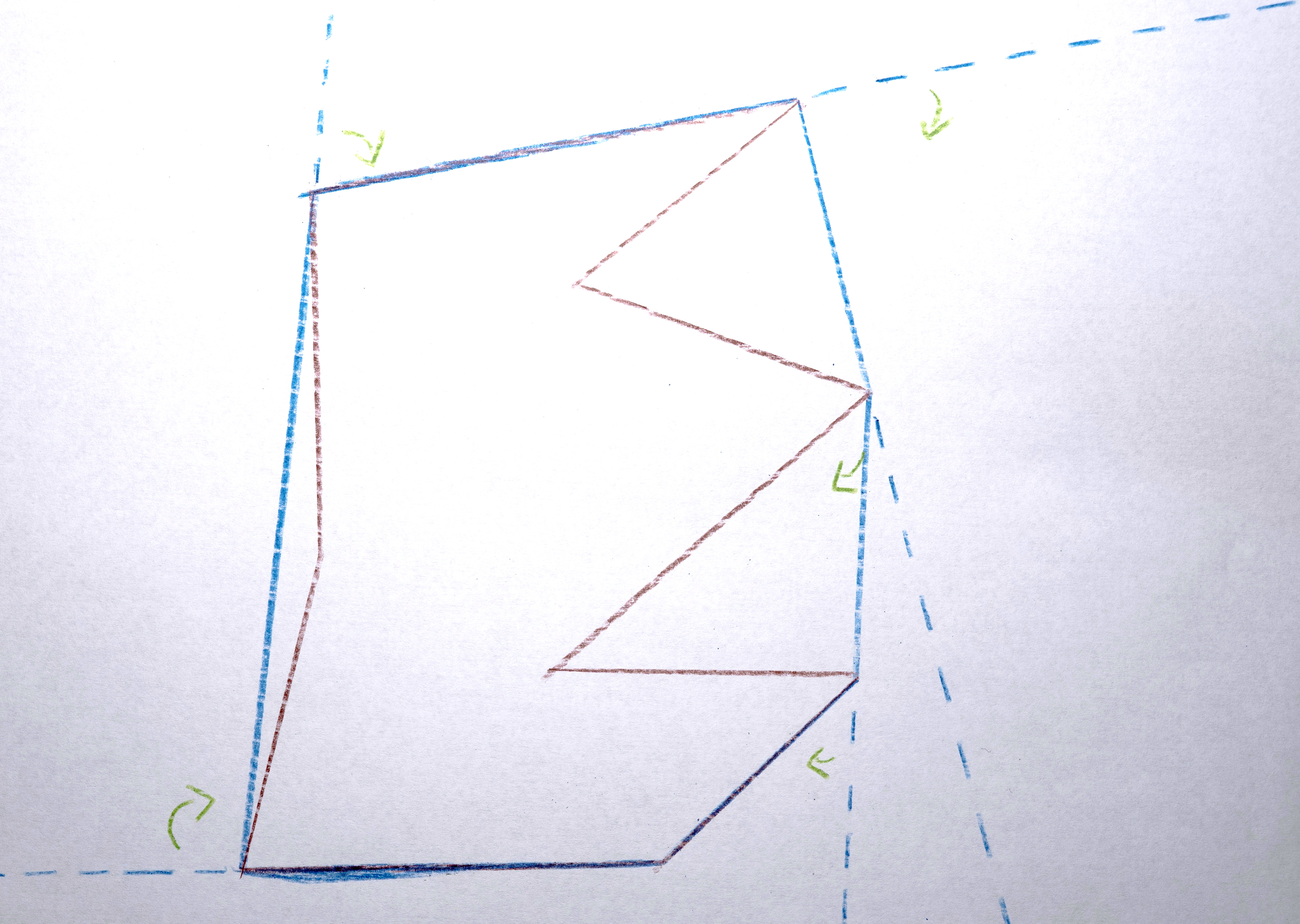
2. Resample each polygon in that sequence to that have that (maximum) number of points creating its perimeter so that when the polygons morph between each other they all have the same number of points to interpolate between.
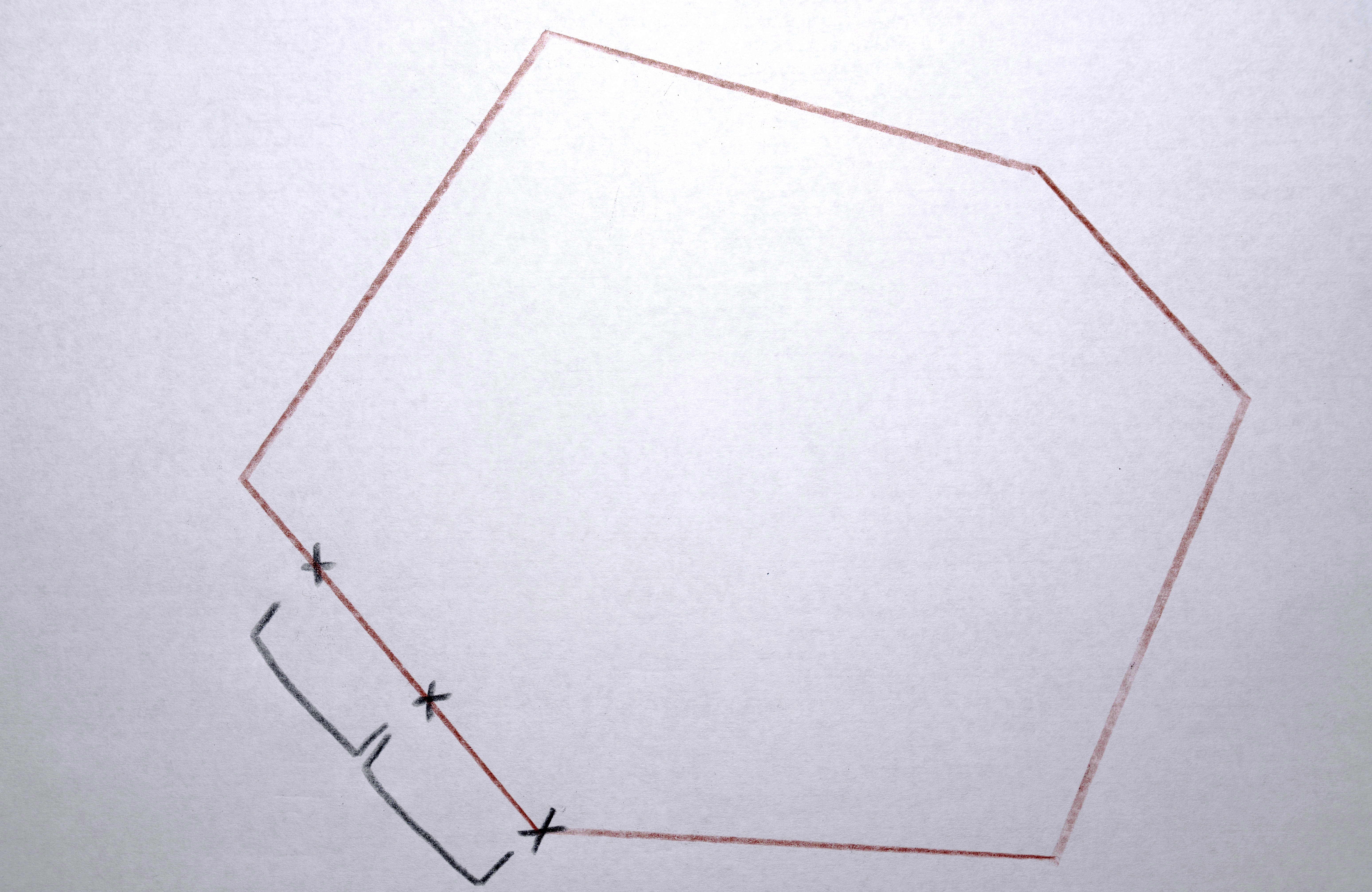
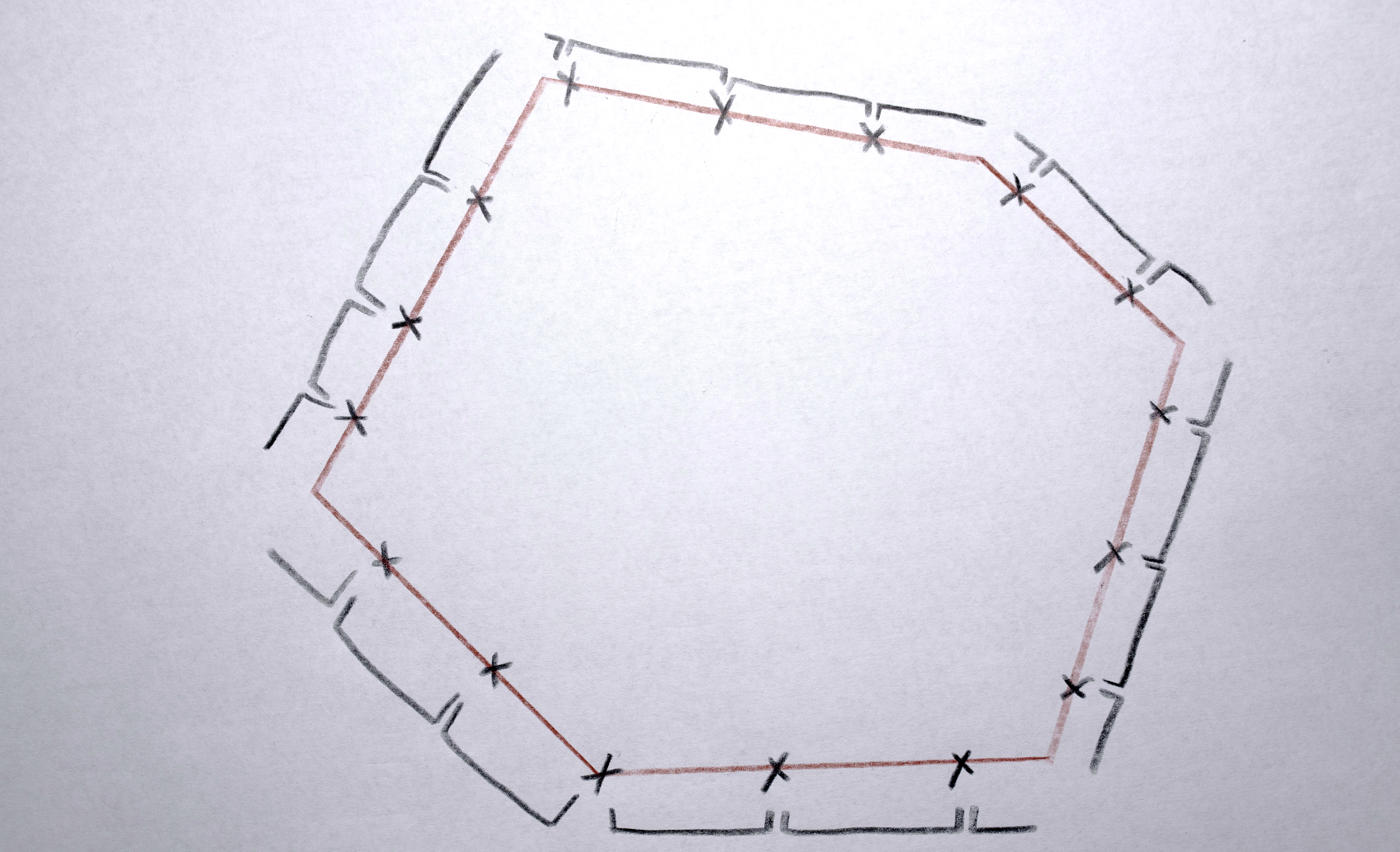
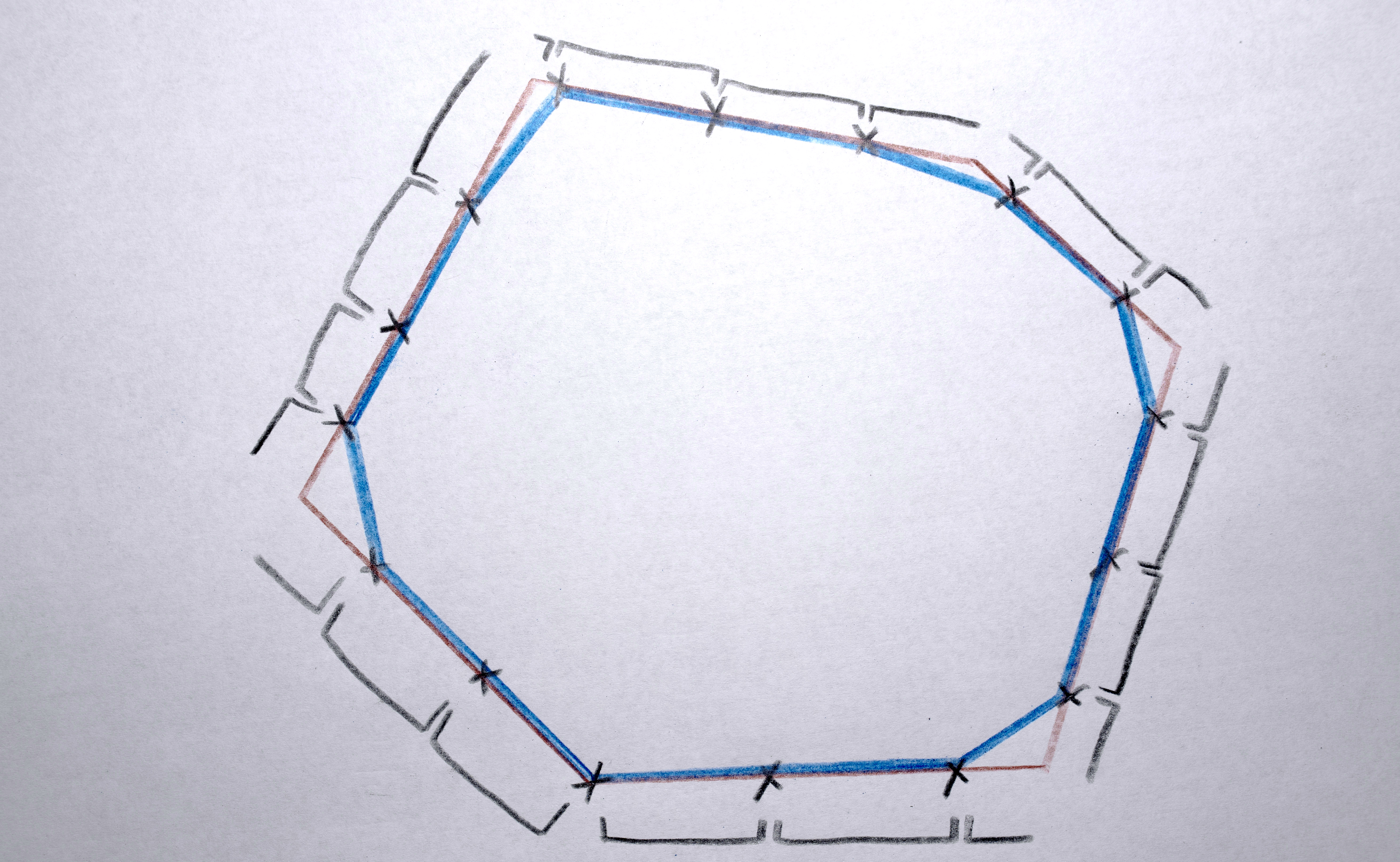
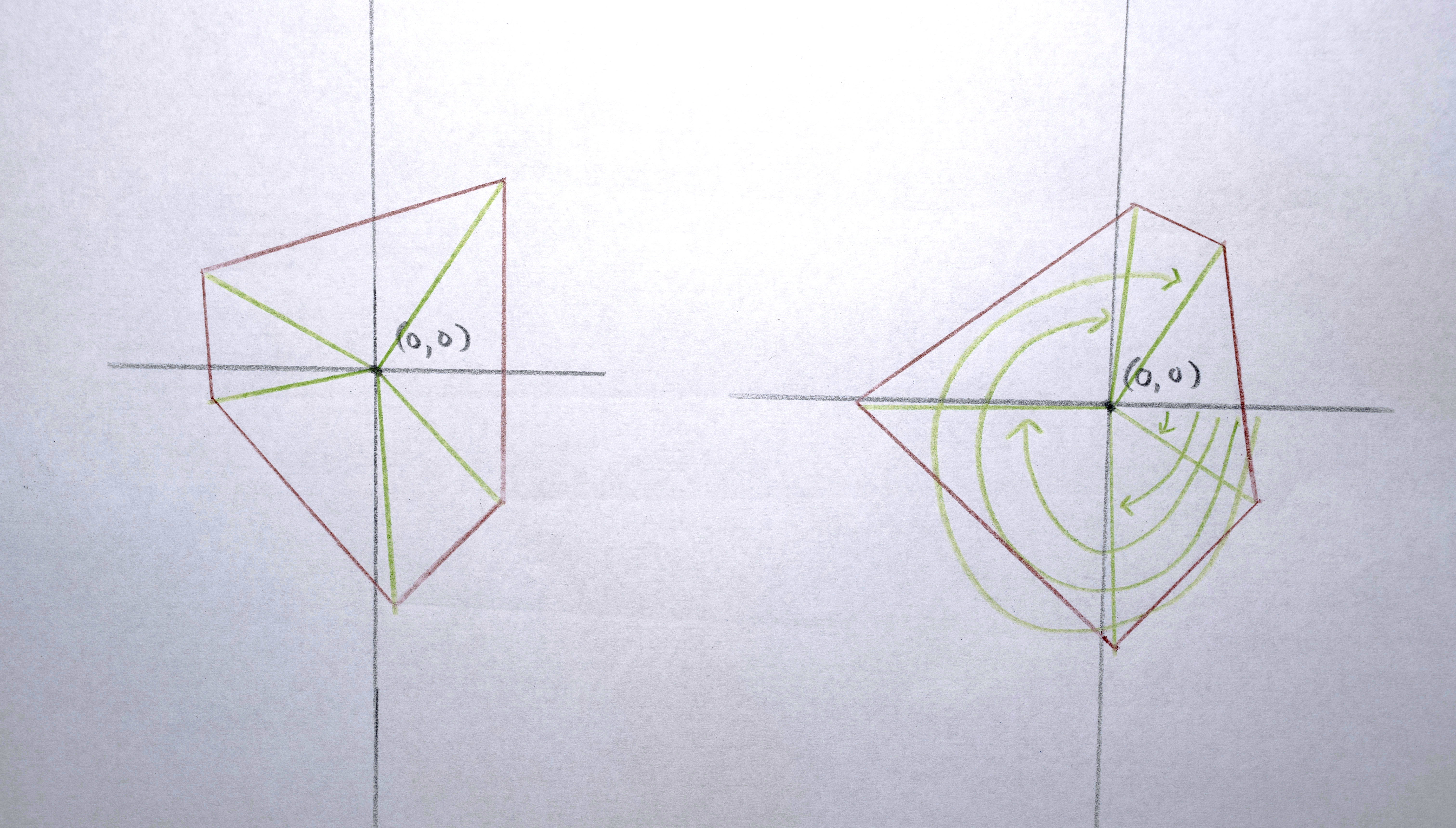
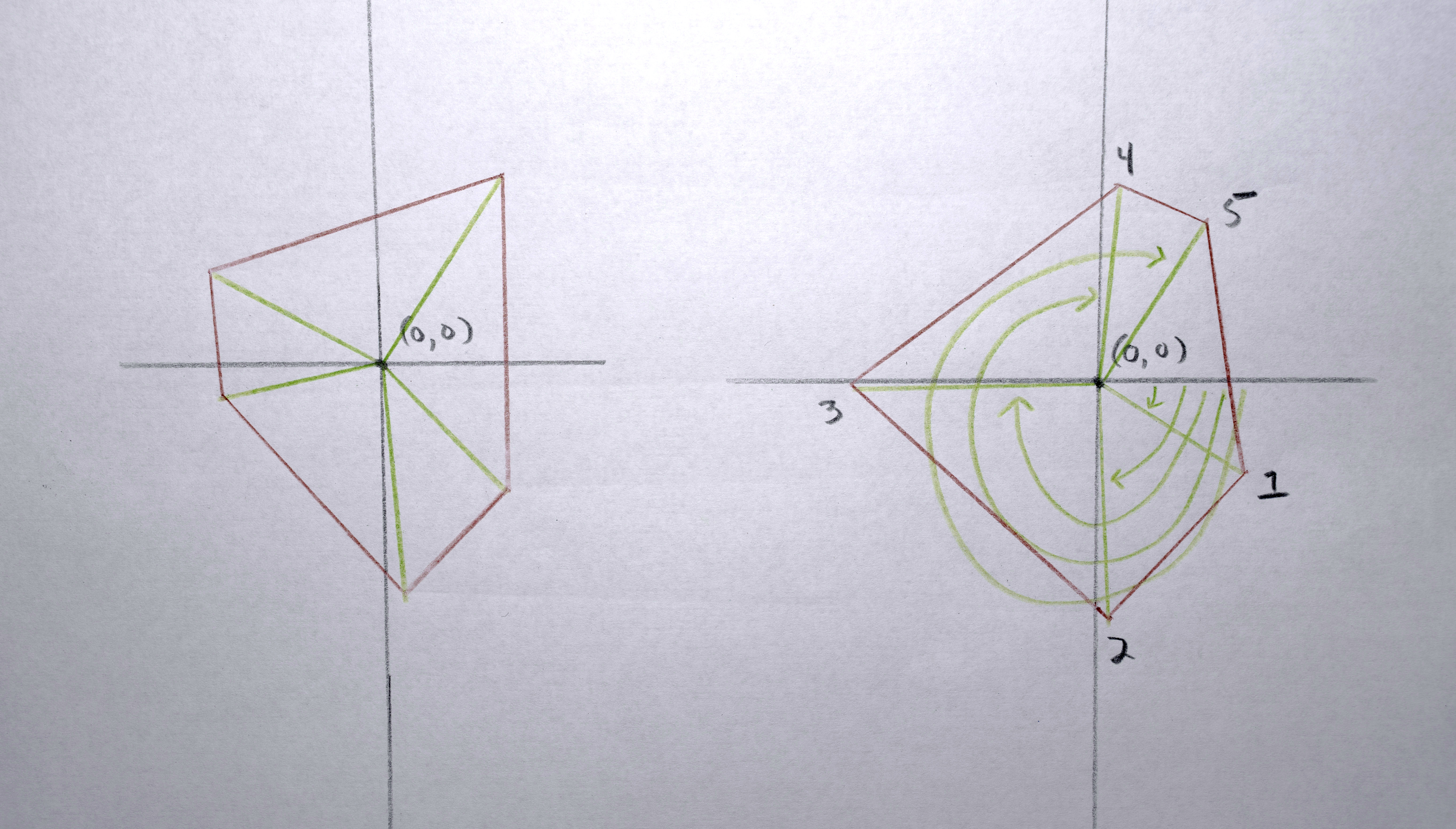
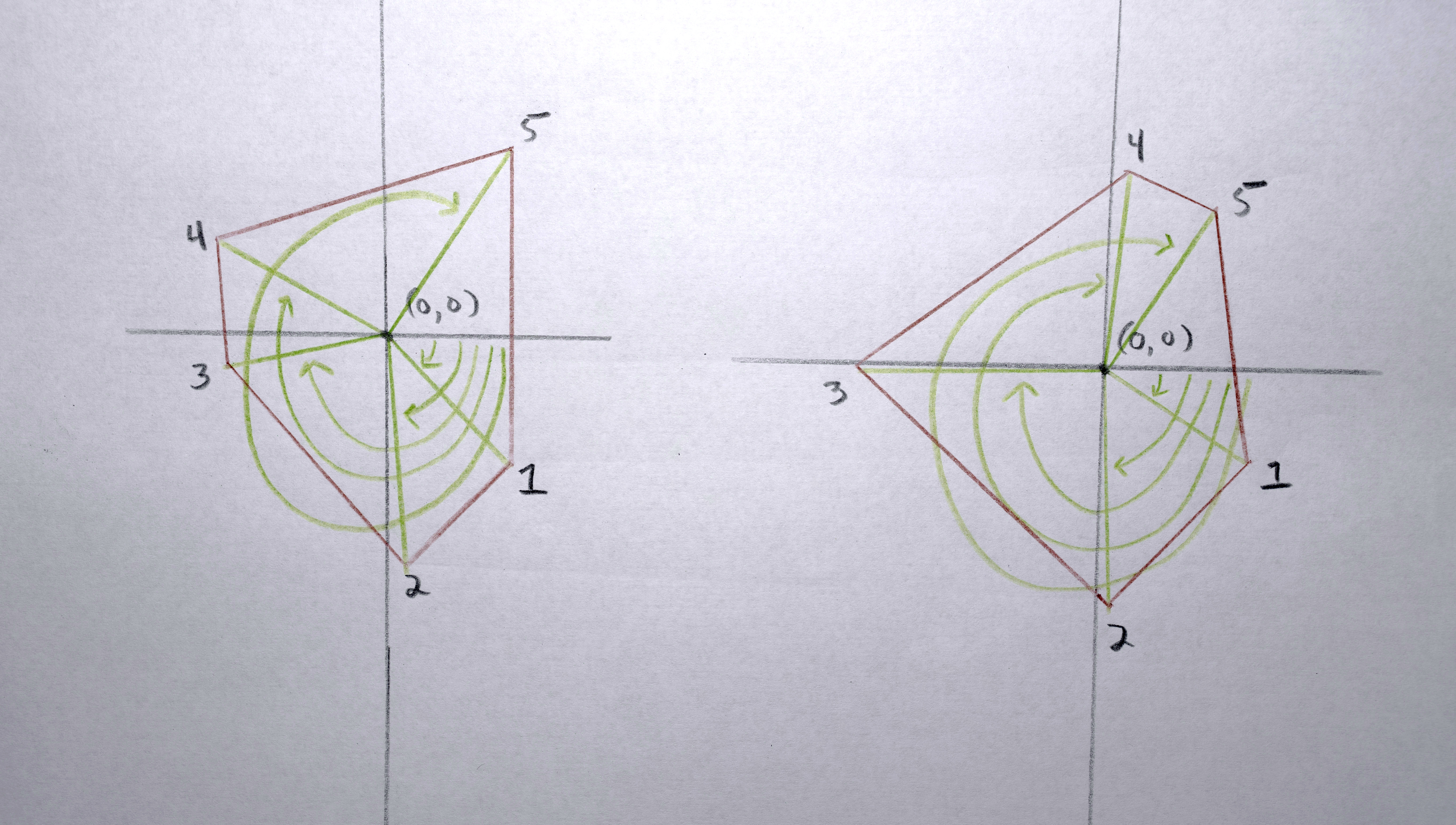
3. Because each polygon is constructed from a list (actually a C++ vector) of points, I need to reorder the points according to their “angle” around the perimeter (by finding the arctangent) so that when the polygons interpolate the points are generally matched up (a point on the left of polygon “a” interpolates to a point on the left of polygon “b”, a point on the top of polygon “a” interpolates to a point on the top of polygon “b”)
Sequence Playback
When I first watched the polygons in all these sequences morphed between each other, they would all “depart” from one position, morph for the same amount of time, and then “arrive” at their next position in synchrony. It looked too robotic for my tastes, so I offset the sequences in time from each other to make a more organic flow.
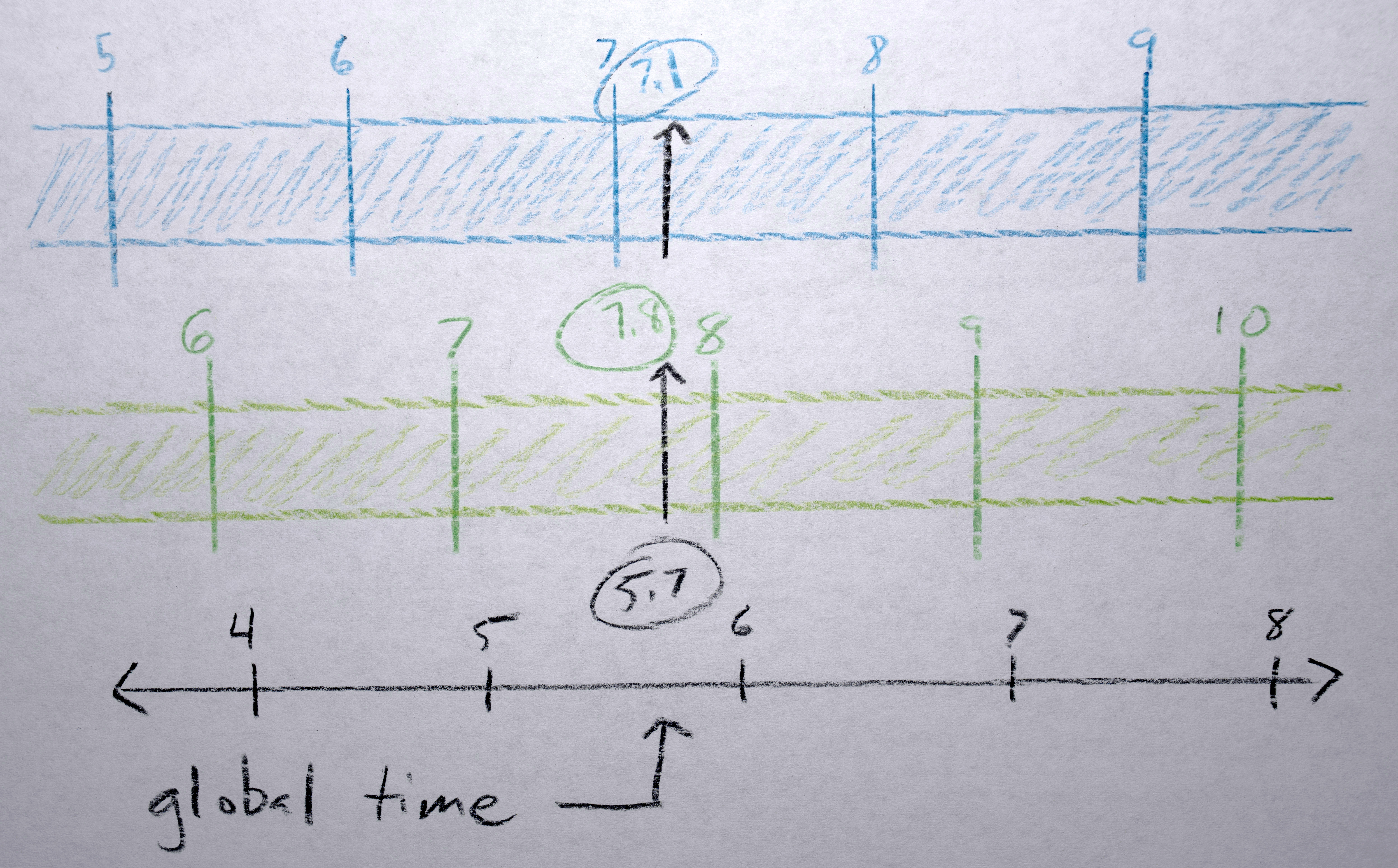
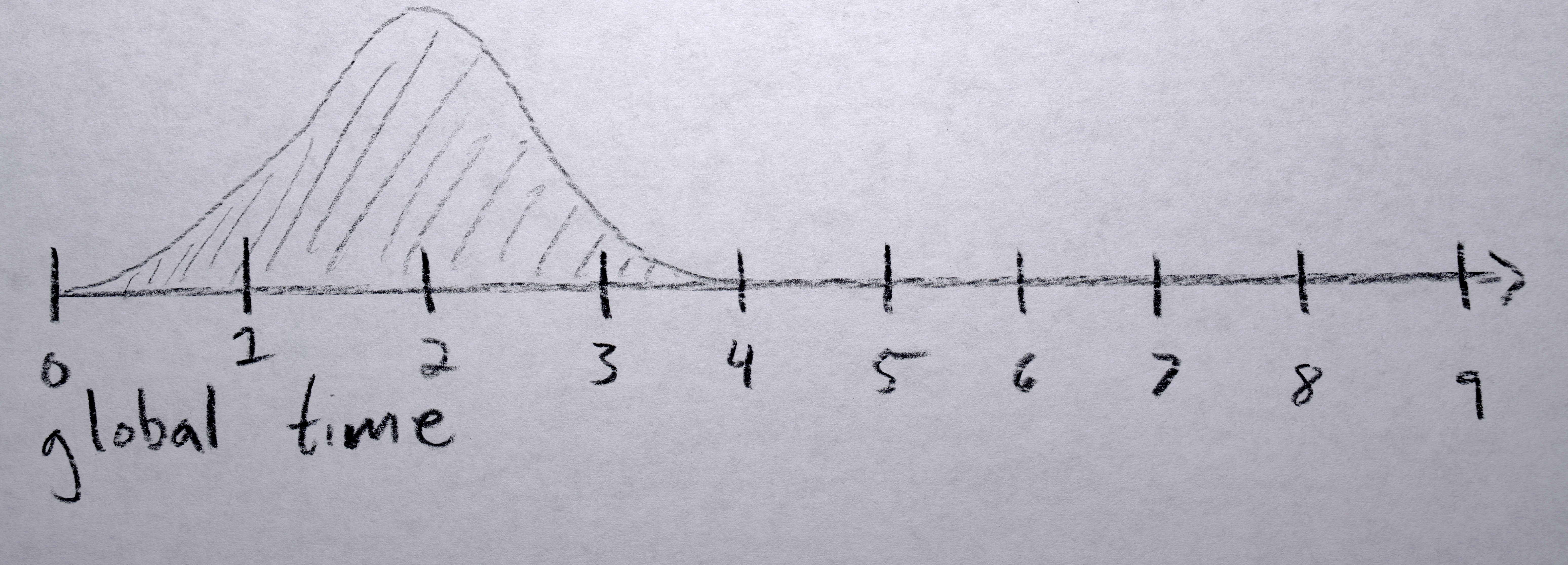
Each polygon gets a “time offset” from a random gaussian distribution with a mean of 0 and standard deviation of 0.5 seconds. Because eventually I would like to have all of these offsets positive (to simplify the code by not needing to worry about negative time), I find the lowest one (which will be negative) and shift each sequence’s time offset up by this much so that the “lowest” time offset will now be zero.
A “global timer” counts forward incrementing 1 / number of interpolations between frames. The global time isn’t counting the number of frames in the final output video, rather it is counting (as integers) the frame numbers of the original analyzed frames, the fractional part between these integers is the interpolation between the analyzed frames. To render each frame of final video, each sequence is passed this global time and adds its unique “time offset”, essentially time traveling it into the future by some amount so it will render “now” what it would look like at that “future” time. Given this position in time (the “offset time”) it checks to see if it, as a sequence, is even active at this time. If it is, it uses the fractional part of the “offset time” position to interpolate between the polygon of the previous integer frame and the next integer frame. The centroid of the polygons is interpolated, moving to a new point on the screen(s) (using monotonic cubic interpolation). The points in each polygon are linearly interpolated between each other (in reference to the centroid, so they move as a whole). The colors of the two polygons interpolate in 3-D, RGB space using s-curve interpolation.

Sequence Birth and Death
When first appearing, a sequence has a “life span” counter that increases every frame that it “has been alive”, which is used to fade the alpha of the color from 0 to full (255) over a set number of frames. When the “offset time” is greater than the last frame of the sequence, (1) the polygon points and color stays fixed according to the last polygon in the sequence, (2) the convex hull centroid continues moving in whatever direction vector was last used (so it looks like “momentum” is naturally carrying it), and (3) the alpha fades out over a defined number of frames.
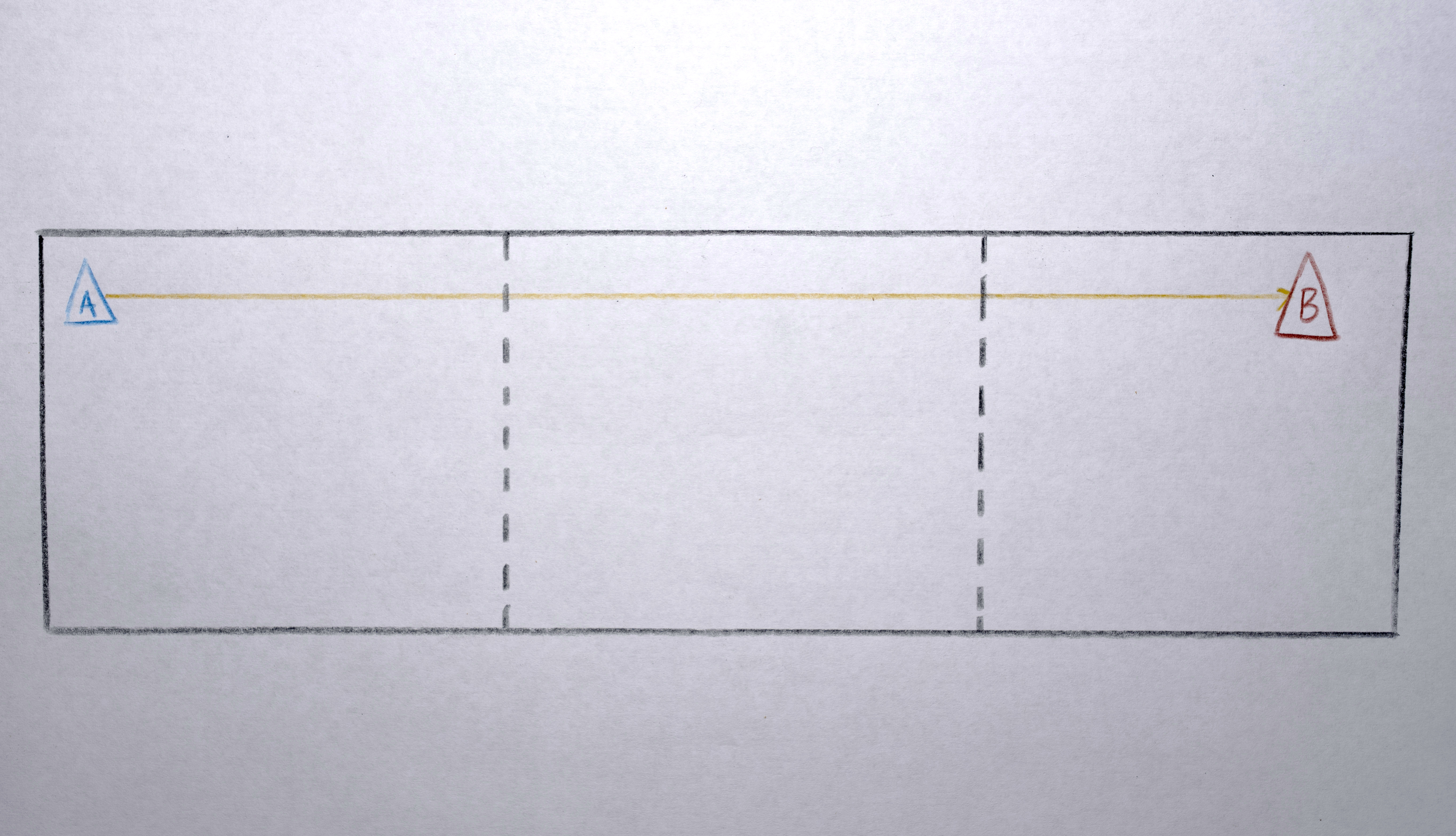
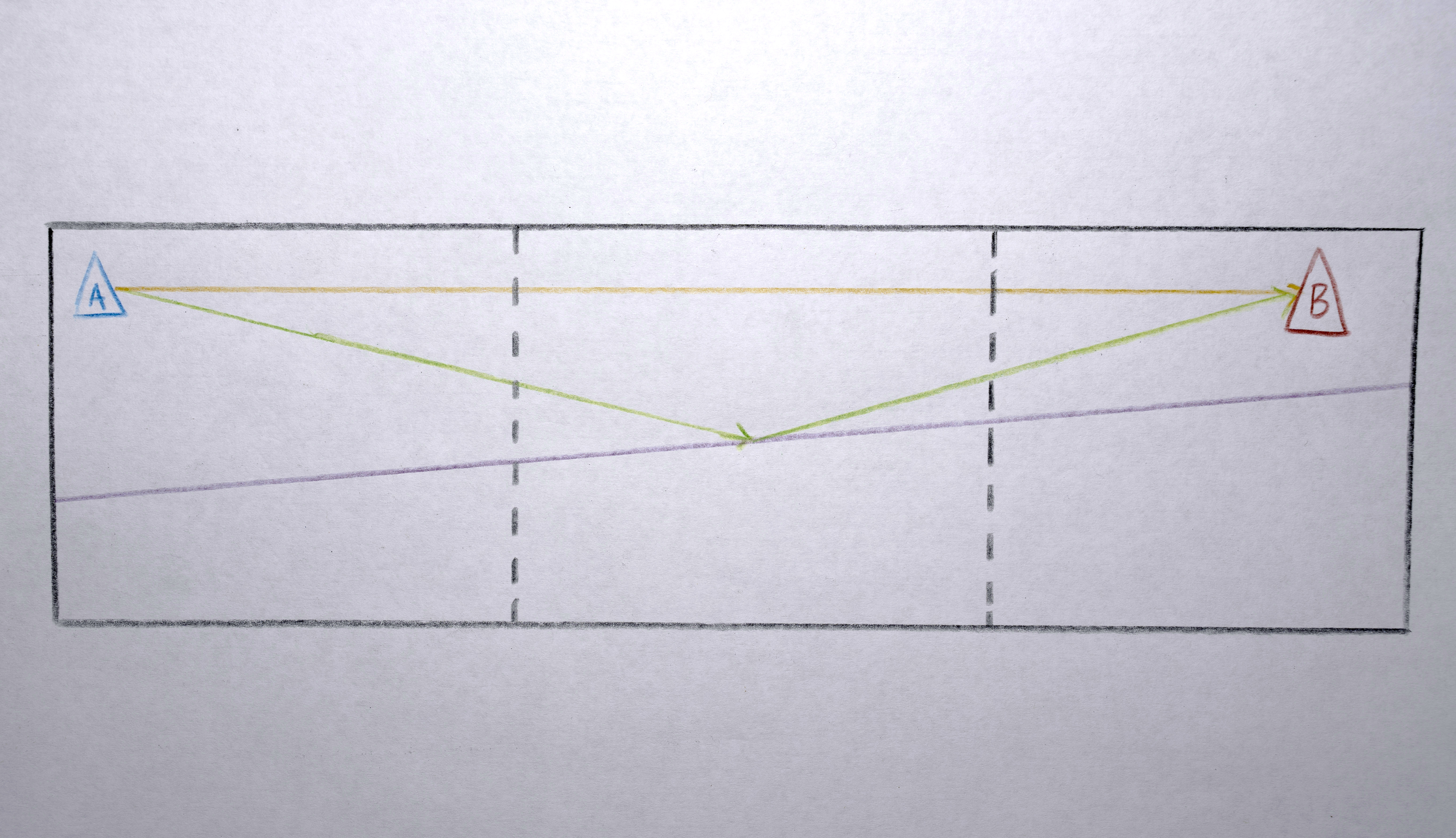
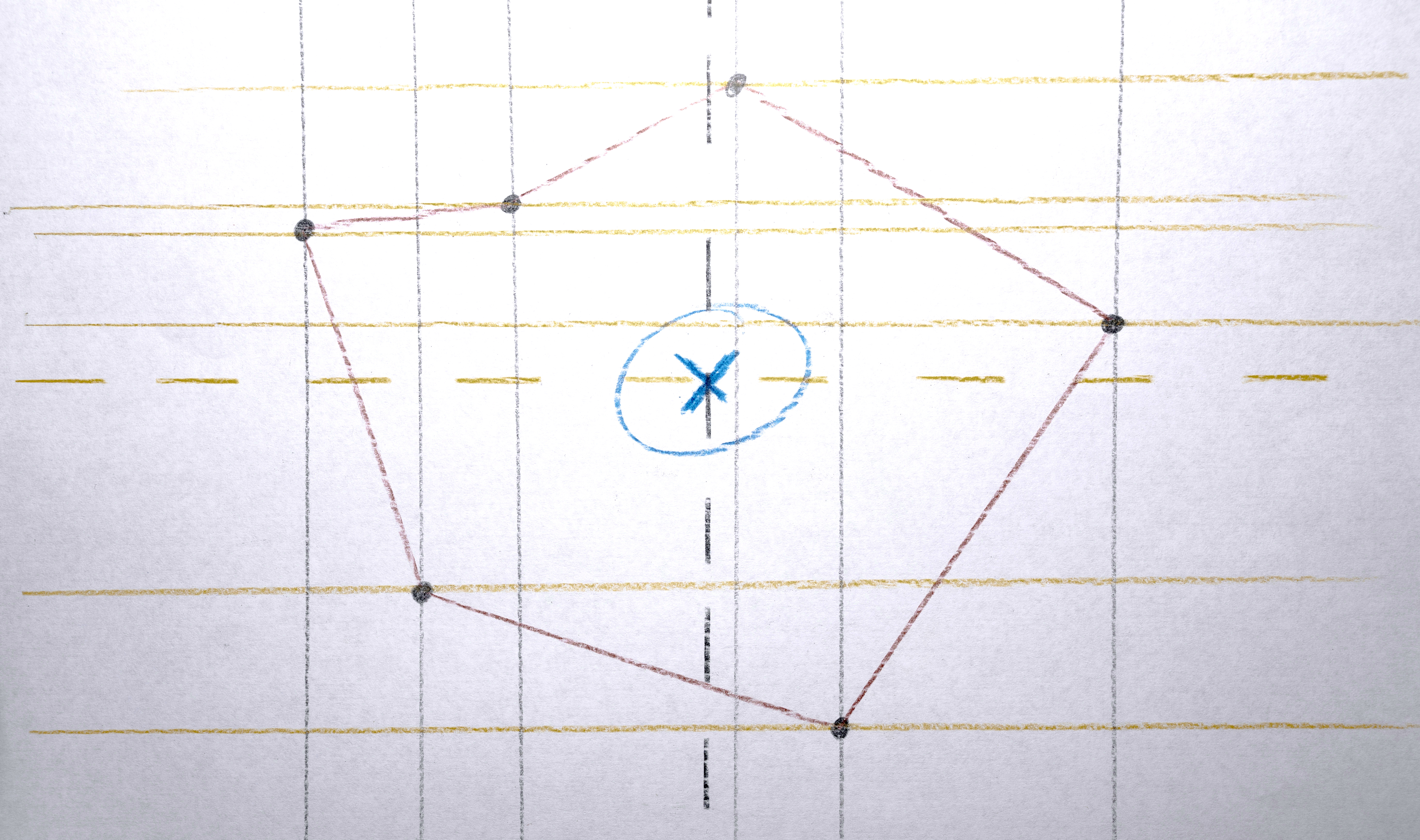
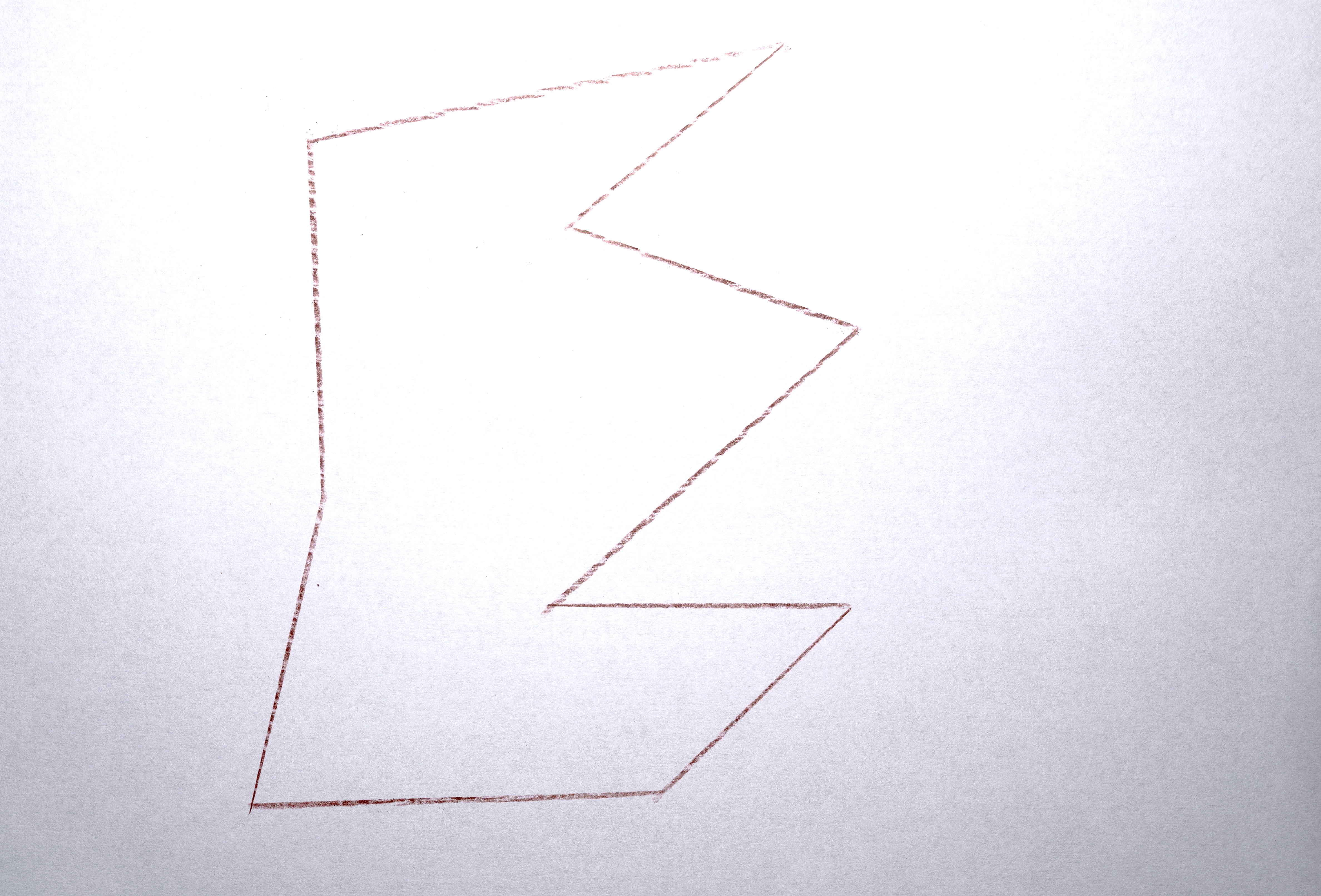
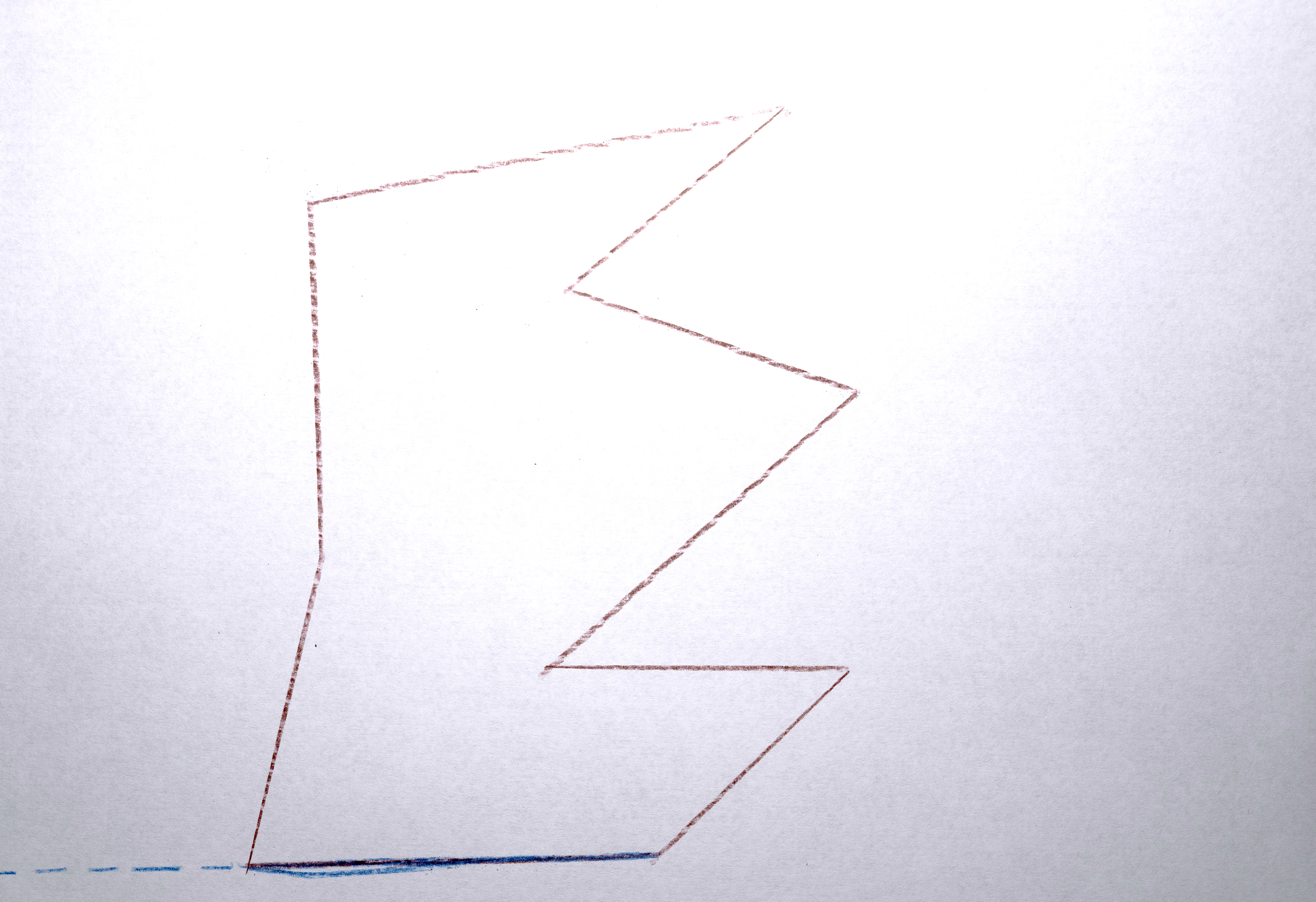
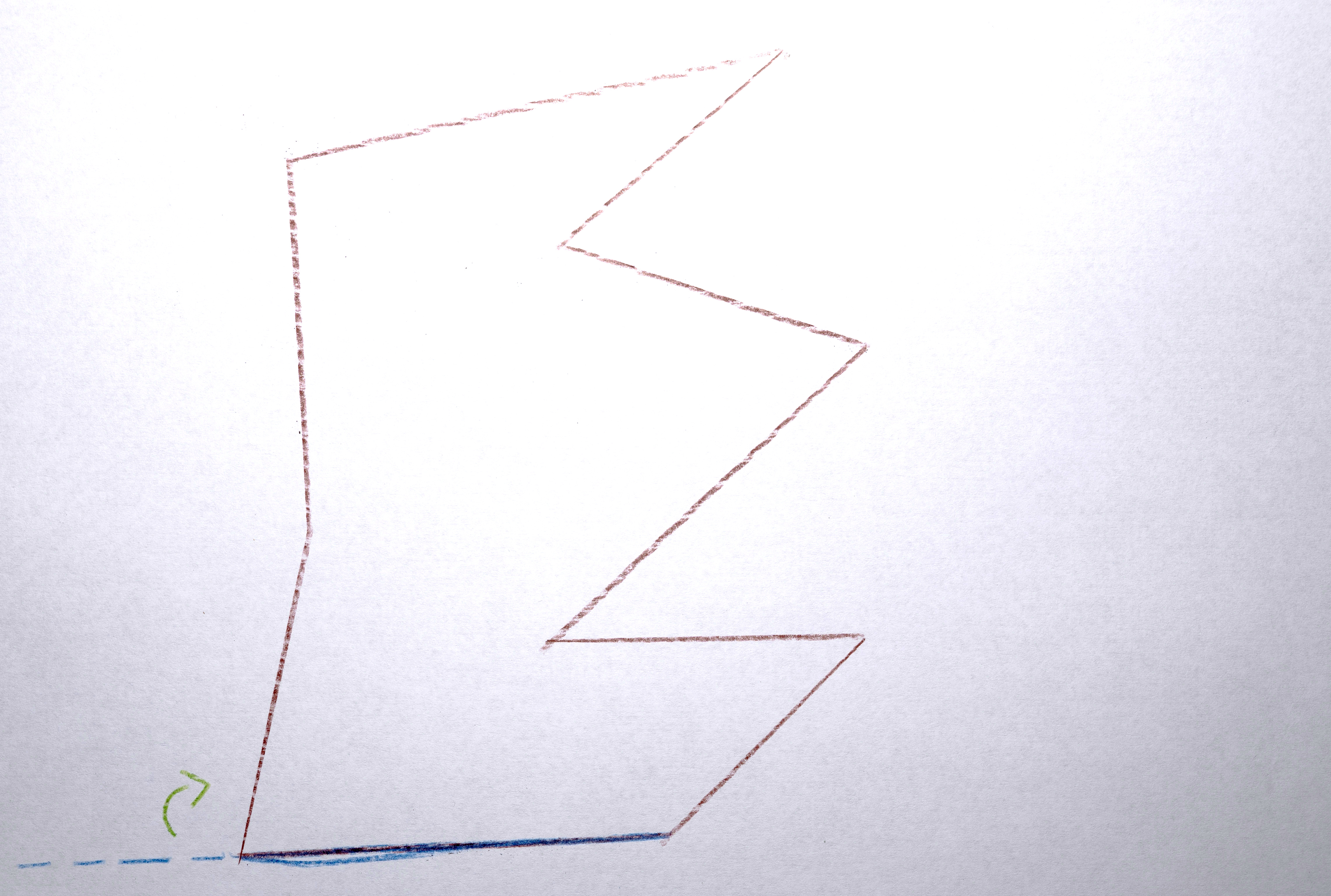
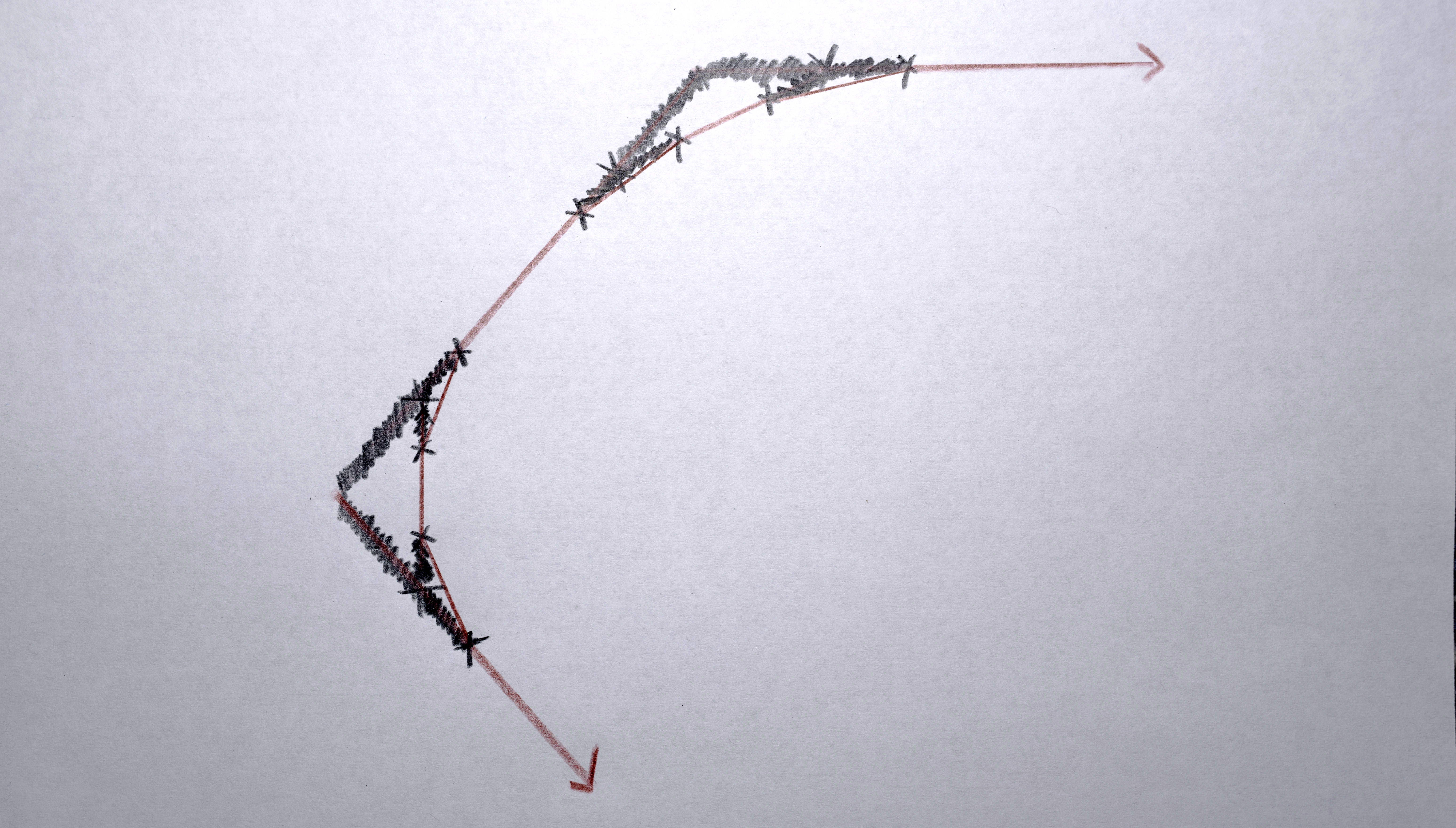
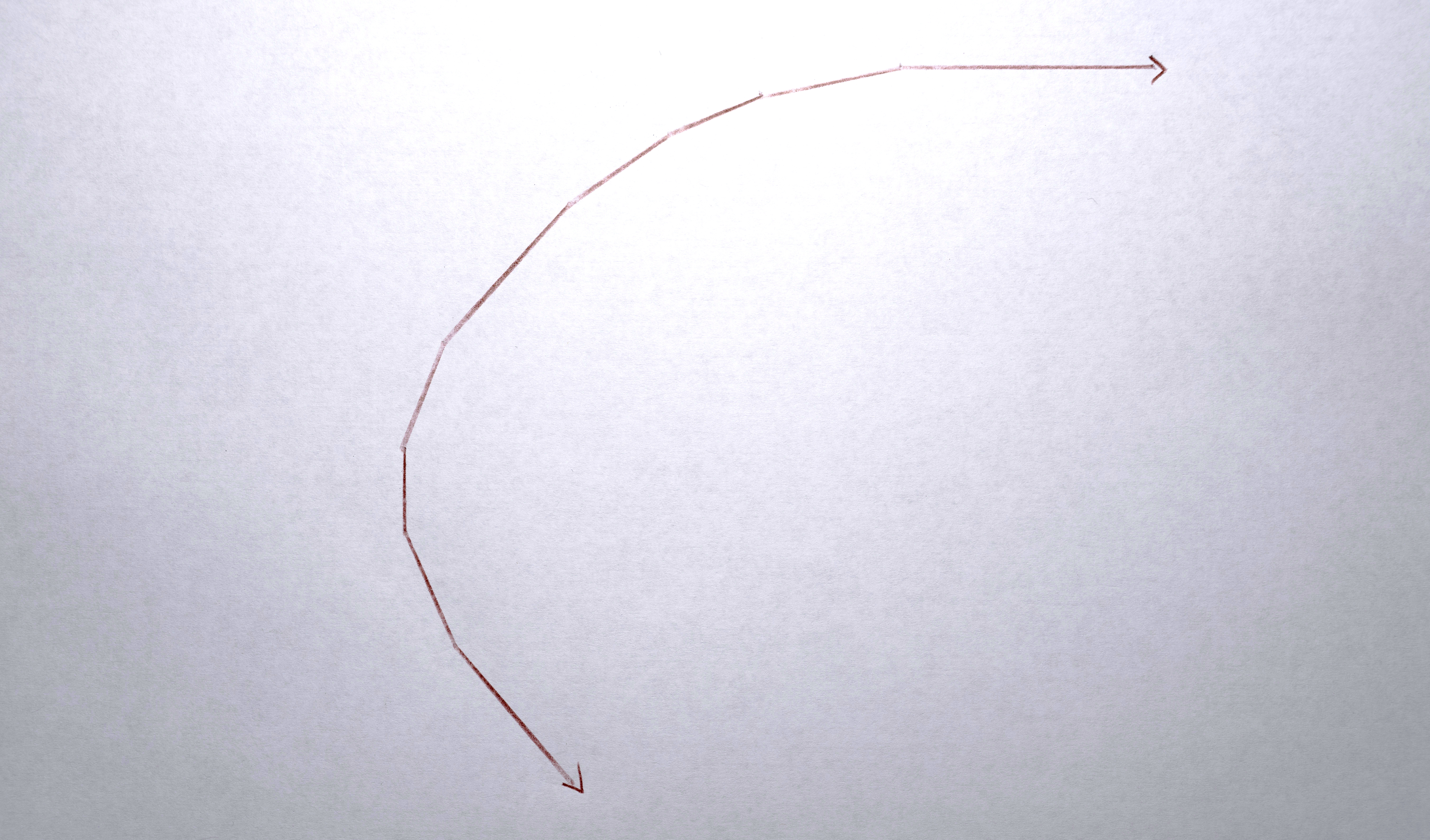
Organic Flows
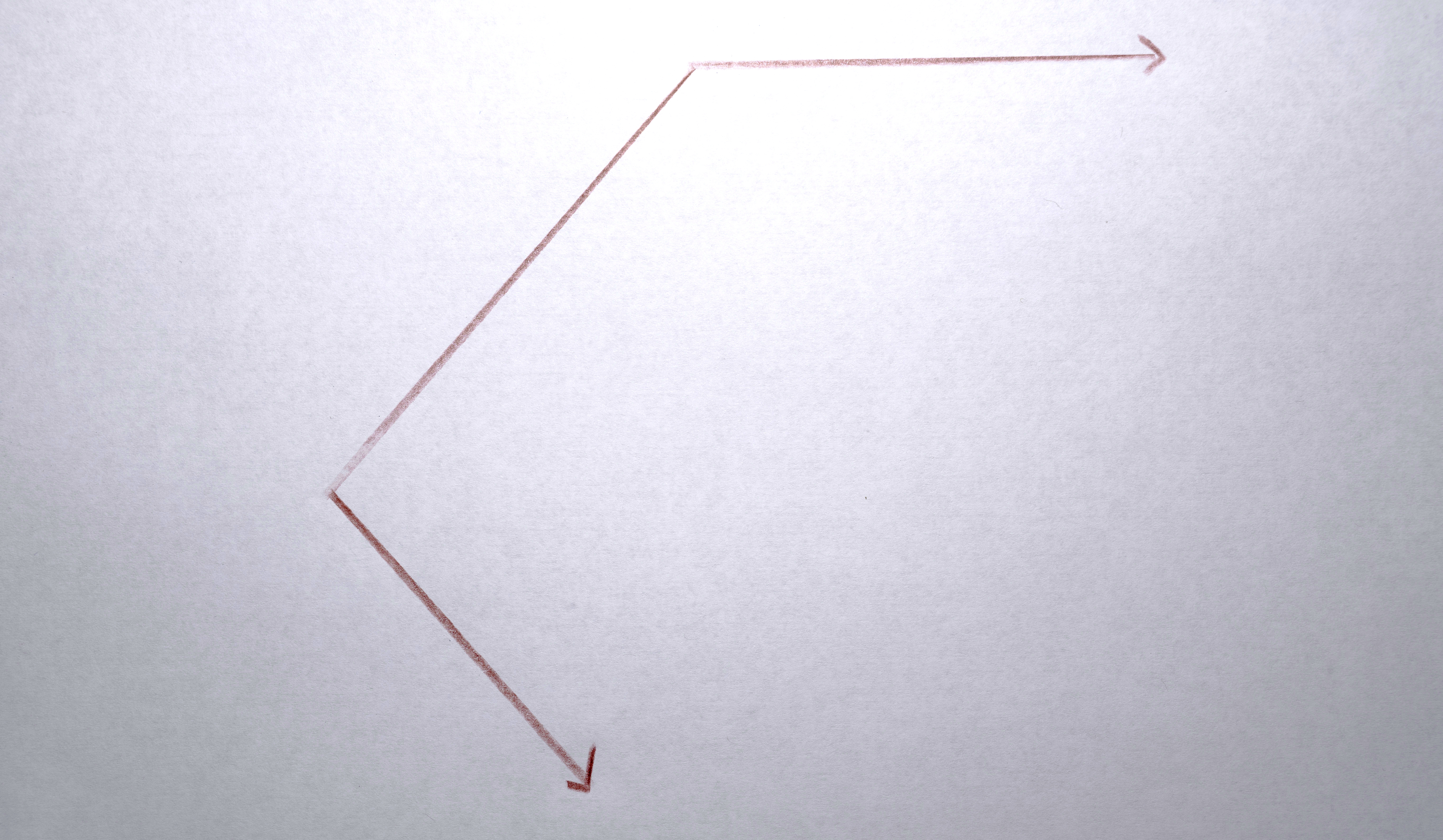
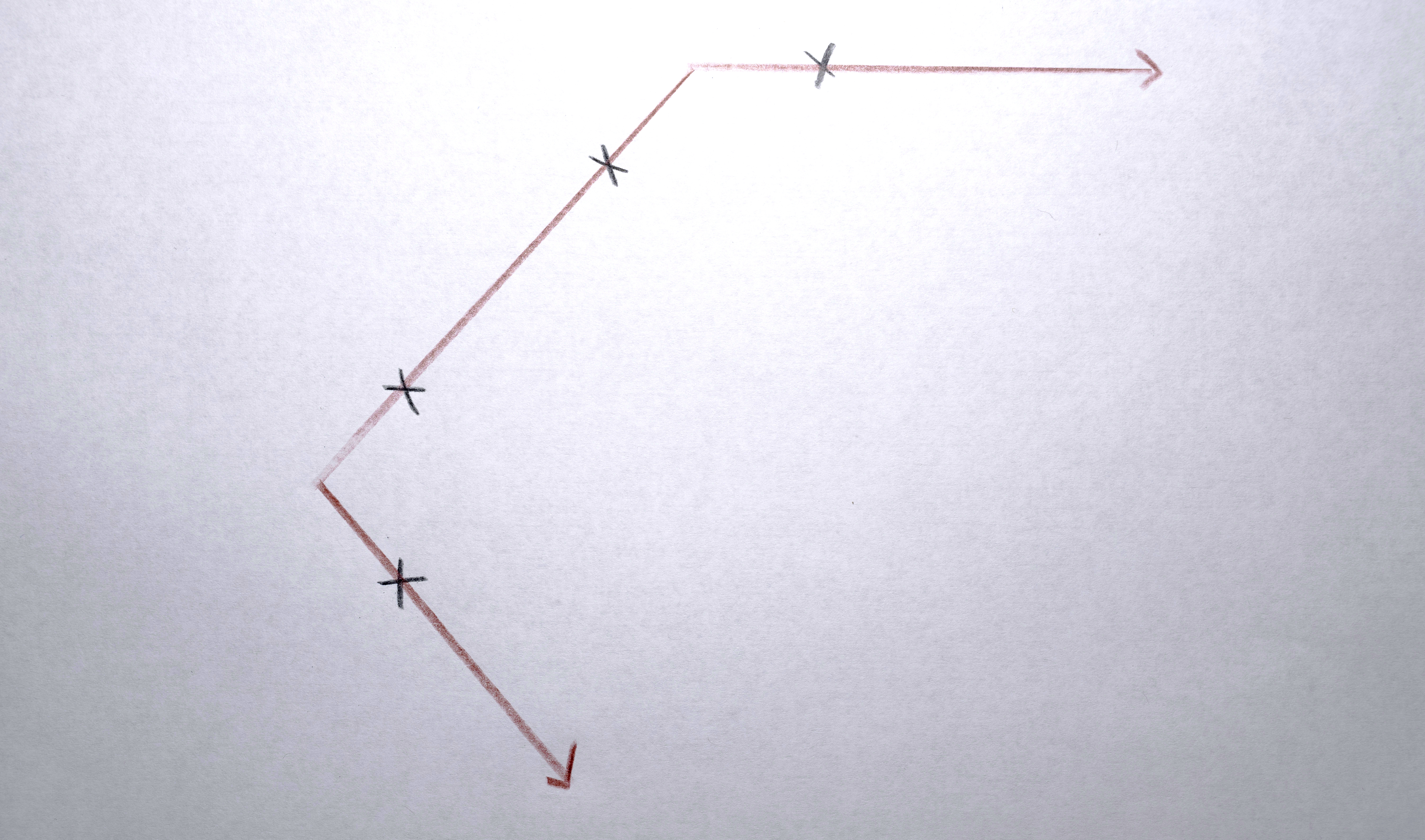
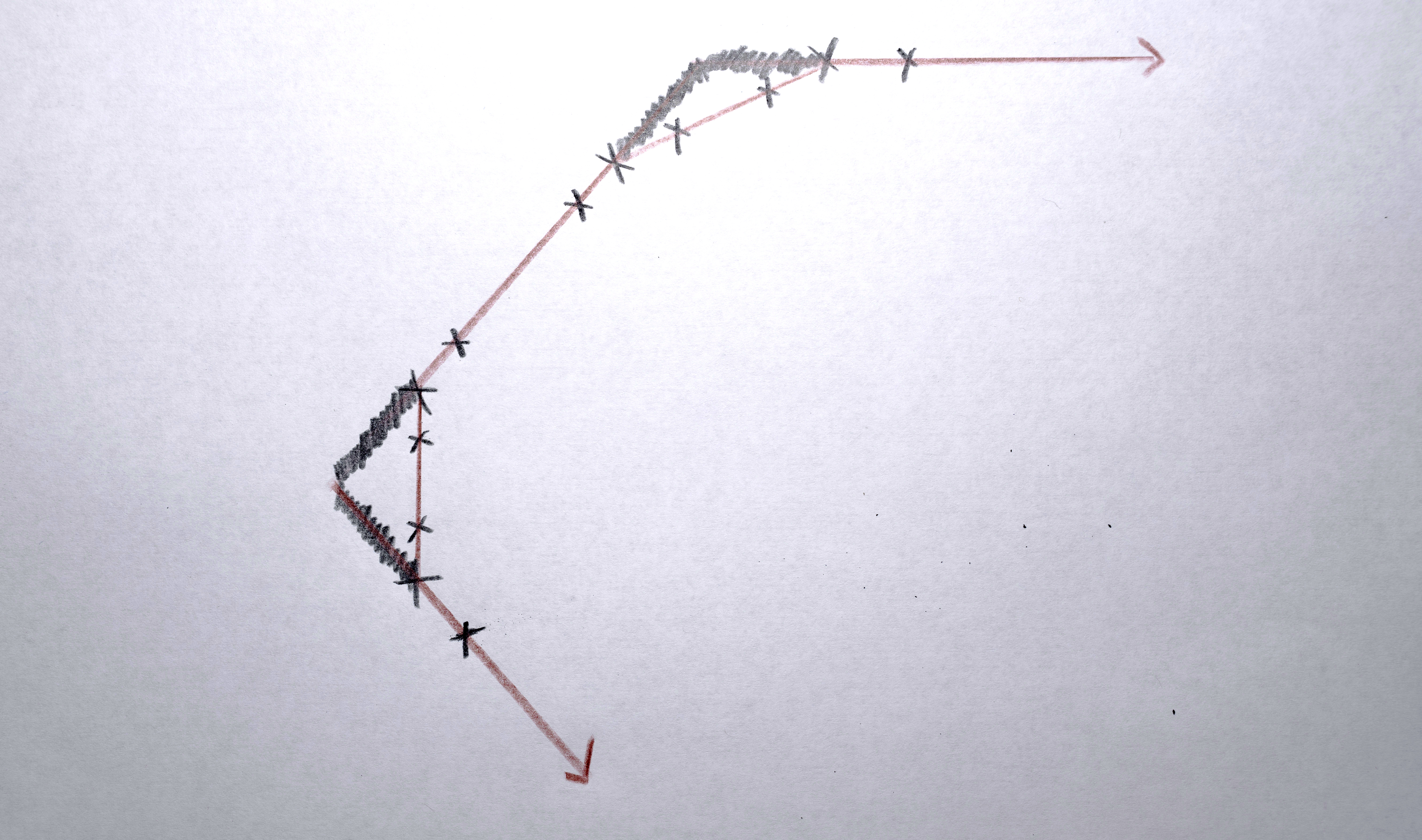
Some of these interpolations don’t shift polygons by small amounts, but rather drag polygons across to a new screen and a new scene. For these interpolations the path from one polygon to the next originally followed a rather straight line which was too “literal” or “robotic”. I wanted the polygons to flow more organically. For these interpolations I implemented a “swerve” by giving each sequence a “secret” line that connects the two sides of the video, mostly centered around the middle (the lines are random, using a gaussian distribution along the y axis). For these big “interpolations,” as the polygon moves from one point to the other it swerves to meet this secret line in the middle of its path, giving it just enough non-direct motion to flow more organically. When all the polygons do this together, the result is quite fluid. The “serving” is executed by using a weighted average between the expected path of the polygon and the path of the “secret” line. Over the course of the interpolation, the centroid of the polygon starts at the expected position, in the middle of the interpolation it hits the “swerve line” (where it is on the y axis at that x position) and by the end of the whole interpolation it is back to the expected position. The weighted average interpolation is created by modifying the 0 to 1 signal of the interpolation to a triangle signal ramp (0 to 1 to 0), then an s-curve transformation is applied so that the peak of the triangle is a hard “bounce” off the “secret” line.